Analysis of multi-condition single-cell data with latent embedding multivariate regression
·Projecting cells into different spaces based on experimental conditions
Eltze and Huber et al (2025) https://doi.org/10.1038/s41588-024-01996-0 found a method on surveying gene differential expressions on multi-condition scRNA-seq. Instead of integrating the cells from different experiments, this paper is proposing a different way to merge the cells and could led to meaningful DE analysis for different conditions.
“The central idea of LEMUR is to represent multi-condition single-cell RNA-seq data using a multi-condition extension of PCA.”
From my understanding, first of all, all the cells were mapped to a common integrated space (the base space). Then the subspace-spanning matrix R were calculated for each condition that could “rotate” the cell coordinates into a particular subspace. Such rotation is implicated in gene differential expressions upon a certain condition (described by the design matrix). And LEMUR then translate the rotation into DEGs by pseudobulk DE test (using EdgeR).
A second important feature that LEMUR renders is that it could project the cell coordinates from the base space back to the condition space, and thus could give us a rough estimate of how the cell would experience DE when change from one condition to another.
This method that provide a full mapping of cells across conditions are definitely useful in many settings and the way it analyses DE also sounds very comprehensive and appears to explain the residual variance very well rather than throwing them away in the integration step. Thus, I think it would worth trying to go through some of the examples and go deeper to learn how to use this package.
Glioblastoma analysis using LEMUR
The glioblastoma dataset was published by Zhao et al, 2020 GSE148842 to study the drug response in human tumour tissues using sc-RNAseq.
It treated the tumor with panobinostat or etoposide, and thus we have 3 treatment condition: ctrl, panobinostat, and etoposide. In the LEMUR tutorial for giloblastoma, we were only focusing on the comparison between ctrl and panobinostat. There were 5 patients (PW030-PW040) that had panobinostat treatments and thus, we have 5 patient conditions.
The design matrix would be like this:
| condition | intercept | etoposide | panobinostat | PW030 | PW032 | PW034 | PW036 | PW040 |
|---|---|---|---|---|---|---|---|---|
| ctrl | 1 | 0 | 0 | 0 | 0 | 0 | 0 | 0 |
| etoposide | 1 | 1 | 0 | 0 | 0 | 0 | 0 | 0 |
| panobinostat | 1 | 0 | 1 | 0 | 0 | 0 | 0 | 0 |
Since, we are not interested in patient-specific expression, we kept all patient column as “0”. In the beginning of the tutorial, most of the efforts were used in putting the sample together as 1 big SingleCellExperiment object.
library(tidyverse)
library(lemur)
library(glue)
library(SingleCellExperiment)
library(monocle3)
library(Matrix)
set.seed(1)
setwd("../../LEMUR_sc_multi_condition/")
file_df <- tibble(file = list.files(path = "../LEMUR_sc_multi_condition/GSE148842_RAW/", full.names = TRUE, pattern= "^GSM"),
                  id = str_match(file, ".+/GSM\\d{7}_(PW[0-9-]*)\\.cts\\.txt\\.gz")[,2])

geo_metadata <- GEOquery::getGEO("GSE148842")
# Parse geo metadata #
patient_annotation <- bind_rows(as_tibble(geo_metadata[[1]]),
                                as_tibble(geo_metadata[[2]])) %>%
  unite("description", starts_with("characteristic"), sep = "\n") %>%
  transmute(id = title, description, origin = source_name_ch1) %>%
  separate(id, into = c("patient_id", "treatment_id"), remove = FALSE) %>%
  mutate(age = as.numeric(str_match(description, "age: (\\d{1,3})\\s")[,2]),
         gender = str_match(description, "gender: ([MF])\\s")[,2],
         location = str_match(description, "location:\\s*([^\\n]+)\\s*\\n")[,2],
         diagnosis = str_match(description, "diagnosis:\\s*([^\\n]+)\\s*\\n")[,2],
         treatment = str_match(description, "treatment:\\s*([^\\n]+)\\s*$")[,2]) %>%
  dplyr::select(-description) %>%
  mutate(patient_id = ifelse(str_starts(id, "PW05"), str_sub(id, start = 1L, end = -4L), patient_id),
         treatment_id = ifelse(str_starts(id, "PW05"), str_sub(id, start = -3L, end = -1L), treatment_id)) %>%
  mutate(origin = ifelse(origin == "glioma surgical biopsy", "biopsy", "tissue_slice"),
         recurrent_tumor = str_ends(diagnosis, "recurrent")) %>%
  mutate(condition = case_when(
    treatment == "vehicle (DMSO)" ~ "ctrl",
    treatment == "2.5 uM etoposide" ~ "etoposide",
    treatment == "0.2 uM panobinostat" ~ "panobinostat",
    .default =  ~ "other",
  ))
### 43 samples, 10 patients, selected 3 treatment conditions for Lemur analysis ###
# Select panobinostat and one random slice for each condition
set.seed(1)
### make a file that have patient metadata and dir path to the scRNA dataset
tmp <- patient_annotation %>%
  tidylog::inner_join(file_df) %>%
  filter(condition != "other") %>%
  filter(! recurrent_tumor) %>%
  filter(origin == "tissue_slice")
### 26 files with different conditions ctrl, ectopside and panobinostat ###

# Load SingleCellExperiment from file
sces <- map(tmp$file, \(fi){
  id <- str_match(fi, ".+/GSM\\d{7}_(PW[0-9-]*)\\.cts\\.txt\\.gz")[2]
  df <- data.table::fread(file = fi, showProgress = FALSE)
  rowdata <- df[,c("gid", "gene")]
  counts <- df %>%
    dplyr::select(- c(gid, gene)) %>%
    as.matrix() %>%
    as("dgCMatrix")
  rownames(counts) <- rowdata$gid
  rownames(rowdata) <- rowdata$gid
  sce <- SingleCellExperiment(list(counts = counts), colData = data.frame(id = rep(id, ncol(counts))), rowData = as.data.frame(rowdata))
  # Reduce to 800 cells per sample
  # sce <- sce[,sample.int(ncol(sce), min(ncol(sce), 800))]
  sce
}, .progress = TRUE)
### combine 26 list of patients to a single experiment ###
sce <- do.call(cbind, sces)
dim(sce)
### 60725 genes x 122548 cells ###
After rbinds all expression matrix together, we ended up with 60725 genes and 122548 cells. Each sample had cells ranging from 1696 to 15894 and here is the breakdowns.
colnames <- make.unique(colnames(sce))
### add patient annotation to sce ###
colData(sce) <- colData(sce) %>%
  as.data.frame() %>%
  tidylog::left_join(tmp, by = "id") %>%
  dplyr::select(- c(file, origin, recurrent_tumor)) %>%
  DataFrame()
sce$pat_cond <- paste0(sce$patient_id, "-", sce$condition)
table(colData(sce)$pat_cond)
#PW029-ctrl    PW029-etoposide         PW030-ctrl    PW030-etoposide PW030-panobinostat
#       1696               4454              21147               3942               7118
#PW032-ctrl    PW032-etoposide PW032-panobinostat         PW034-ctrl    PW034-etoposide
#        7647               2508               1401              15288              15894
#PW034-panobinostat         PW036-ctrl    PW036-etoposide PW036-panobinostat         PW040-ctrl
#          2679              13289               6120               3096              14282
#PW040-panobinostat
# 1987
Then we proceeded with the filtering (genes have counts in >=5 cells) and transformation (log-transform). Then we removed cells based on qc_df that cells with high mitochondria portions were removed. Finally, we removed cells that have abnormally high read counts, only keeping cells that have total read counts between 800 and 1200.
logcounts(sce) <- transformGamPoi::shifted_log_transform(sce)
colnames(sce) <- colnames
# Remove useless genes
sce <- sce[rowSums(counts(sce)) >= 5, ]
## 37276 genes x 122548 cells ###
# Remove version number of ENSEMBL gene id's
rowData(sce)$gid <- stringr::str_remove(rowData(sce)$gid, "\\.\\d+")
rownames(sce) <- rowData(sce)$gid

qc_df <- scuttle::perCellQCMetrics(sce, subsets = list(Mito = ! is.na(rowData(sce)$chromosome) & rowData(sce)$chromosome == "MT",
                                                       Y_chr = ! is.na(rowData(sce)$chromosome) & rowData(sce)$chromosome == "Y"))


as_tibblssceas_tibblsceas_tibble(qc_df, rownames = "barcode") %>%
  tidylog::left_join(as_tibble(colData(sce), rownames = "barcode"), by = "barcode") %>%
  group_by(patient_id, gender) %>%
  summarize(max(subsets_Y_chr_percent))

summary(qc_df$sum)
summary(qc_df$detected)
summary(qc_df$subsets_Mito_percent)

qc_filters <- scuttle::perCellQCFilters(qc_df, sub.fields = c("subsets_Mito_percent"))
rownames(qc_filters) <- rownames(qc_df)
### no colnames (cell names) were saved though in sce
qc_filters %>%
  as_tibble() %>%
  group_by(across(low_lib_size:high_subsets_Mito_percent)) %>%
  summarize(n = n())
# A tibble: 2 × 4
# Groups:   low_lib_size, low_n_features [2]
#low_lib_size low_n_features high_subsets_Mito_percent      n
#<otlr.flt>   <otlr.flt>     <otlr.flt>                 <int>
#  1 FALSE        FALSE          FALSE                     121545
#  2 FALSE        TRUE           FALSE                       1003
### so 121545 pass QC and 1003 do not due to low features ###
sce <- sce[,!qc_filters$discard]
# Filter out extreme cell sizes
sce <- sce[,colSums(counts(sce)) > 800 & colSums(counts(sce)) < 12000]
qs::qsave(sce, "glioblastoma_cleaned_sce.qs")
Next, the authors utilized the fact that the tumors had a chromosome 7 duplication and a chromosome 10 deletion to define tumor cells.
### look into chromosome 7 duplication and chr 10 deletion ###
### calculate expression level of chr 7, 10 vs chr 1-5 (normal))
sel_chromosomes <- as.character(1:5)
special_chr <- c("7", "10")
w<-deframe(vctrs::vec_group_loc(rowData(sce)$chromosome.y))
w[unique(c(sel_chromosomes, special_chr))]
### identify rows that are in the respecitive chromosome based on rowData ###
### take row Means from counts(sce) ###
chr_counts <- t(lemur:::aggregate_matrix(t(counts(sce)),
            group_split = deframe(vctrs::vec_group_loc(rowData(sce)$chromosome.y))[unique(c(sel_chromosomes, special_chr))], rowMeans2))
rownames(chr_counts)
dim(chr_counts)
### 7 chromosome x 94796 genes ##
ratio7 <- chr_counts["7", ] / colMeans2(chr_counts, rows = 1:5)
ratio10 <- chr_counts["10", ] / colMeans2(chr_counts, rows = 1:5)
simple_label <- ifelse(ratio10 < ratio7, "tumor", "microenvironment")
### so tumor cells have chr7 duplication and chr10 deletion ###
tibble(chr10 = ratio10, chr7 = ratio7) %>%
  mutate(simple_label) %>%
  ggplot(aes(x = chr10, y = chr7)) +
  geom_point(aes(color = simple_label), size= 0.1, stroke = 0) +
  scale_x_log10() + scale_y_log10() +
  guides(color = guide_legend(override.aes = list(size = 1)))
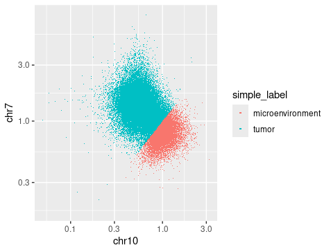
Now, we identified HVG and build PCA and integrated map of the cells. Next, a integrated mapping was built using Harmony with the PCA results.
### HVG ###
set.seed(1)
hvg <- order(-rowVars(logcounts(sce)))
### build pca using 2000 HVG to 35 PC on 94796 cells ###
### res <- prcomp(t(Y), rank. = n, center = center_ind, scale. = FALSE) ###
### list(coordsystem = unname(res$rotation), embedding = unname(t(res$x)), offset = center) ###
subset_pca <- lemur:::pca(logcounts(sce)[hvg[1:2000], ], n = 35)
### run harmony ###
harm <- harmony::RunHarmony(t(subset_pca$embedding), meta_data = colData(sce), vars_use = c("pat_cond", "treatment_id"), lambda = c(1,1))
### harmony embedding show 94796 cells x 35 PC ###
harm_umap <- uwot::umap(harm)
### generate Clustering based on harmony mapping
graph <- bluster::makeKNNGraph(harm, k = 15, BNPARAM = BiocNeighbors::AnnoyParam())
clustering <- igraph::cluster_walktrap(graph)
set.seed(1)
clusters <- igraph::cut_at(clustering, 4)
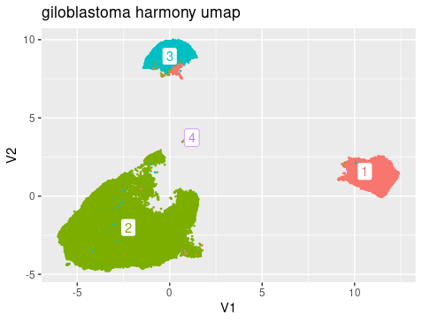
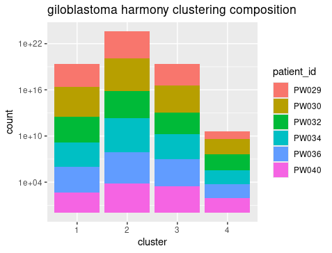
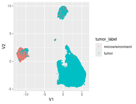
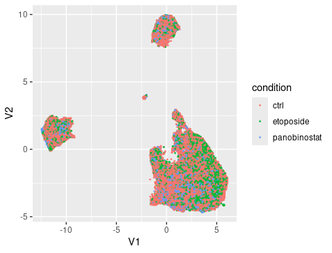
The umap generated from harmony PC showed that there were roughly 4 clusters, reflecting the 4 cell types Myeloid cell, Tumor cells, Oligodendrocytes, and T cells. Breaking down the cell composition per cluster, we can see that the integration is successfully that the patient’s cells are distributed evenly in each cluster. And we can also see that the clustering showed mixing of drug treatment condition and tumor/microenviroment cells. In other words, the clustering reflect mainly the cell type signals but not the treatment or tumor signals.
Differential expression analysis
Here in the tutorial LEMUR github, marker genes were used to QC the clustering. After that, we run LEMUR. Using top 3000 HVG, LEMUR were run based on the design of ** ~ condition + patient_id ** to generate 60 latent embedding for the cells. Finally, we run lemur::test_de and lemur::find_de_neighborhoods to test DEG using aggregated reads from each neighborhood between the ctrl ~ panobinostat condition.
sel_genes <- c("CD14", "TYROBP", "PLP1", "MAG", "TRBC1", "TRBC2", "GAP43")
gene_ids <- deframe(as_tibble(rowData(sce)[c("gene", "gid")]))[sel_genes]
expr_mat <- counts(sce)[gene_ids, ]
cell_type_label <- case_when(
  clusters == 1 ~ "Myeloid cells",
  clusters == 2 ~ "Tumor cells",
  clusters == 3 ~ "Oligodendrocytes",
  clusters == 4 ~ "T cells"
)
colData(sce) <- colData(sce) %>%
  as_tibble() %>%
  mutate(cell_type = cell_type_label, chr_ratio_label = simple_label,
         chr_10_ratio = ratio10, chr_7_ratio = ratio7) %>%
  DataFrame()
reducedDim(sce, "PCA") <- t(subset_pca$embedding)
set.seed(1)
reducedDim(sce, "UMAP") <- uwot::umap(t(subset_pca$embedding))
reducedDim(sce, "harmony") <- harm
reducedDim(sce, "harmony_umap") <- harm_umap
qs::qsave(sce, "glioblastoma_annotated_sce.qs")

sce<-qs::qread("glioblastoma_annotated_sce.qs")
hvg <- order(-rowVars(logcounts(sce)))
#### reduce sce to only contain HVG ###
sce <- sce[hvg[1:3000],]
set.seed(1)
### run lemur to fit the latent embedding model ###
fit <- lemur::lemur(sce, design = ~ condition + patient_id, n_embedding = 60, test_fraction = 0.5)
reducedDim(fit, "fit_umap") <- uwot::umap(t(fit$embedding))

set.seed(1)
### Enforce additional alignment of cell clusters beyond the direct differential embedding ###
fit <- lemur::align_harmony(fit)
### Predict log fold changes between conditions for each cell ###
fit <- lemur::test_de(fit, contrast = cond(condition = "panobinostat") - cond(condition = "ctrl"), new_assay_name = "DE_panobinostat")
qs::qsave(fit, "glioblastoma_fit_hvg3k.qs")

nei_pan <- lemur::find_de_neighborhoods(fit, group_by = vars(patient_id, condition),
                                        de_mat = assay(fit, "DE_panobinostat"), test_method = "edgeR")

qs::qsave(nei_pan, "glioblastoma_fit_hvg3k-nei_pan.qs")
#>  nei_pan
#              name n_cells sel_statistic         pval    adj_pval  #f_statistic df1      df2
#1  ENSG00000210082   91752    -278.19109 6.122879e-02 0.143281094  4.245333375   1 12.26472
#2  ENSG00000118785   87673    -140.95765 2.133515e-02 0.070724261  6.957071366   1 12.26472
#3  ENSG00000167996   59399     -33.45591 9.125650e-02 0.188908456  3.358030447   1 12.26472
#4  ENSG00000087086   82175     -61.24831 3.492159e-01 0.488413852  0.947288731   1 12.26472
#5  ENSG00000120885   91981     153.77459 5.405079e-02 0.131085186  4.537991245   1 12.26472
#6  ENSG00000125148   83114     499.28694 1.781635e-05 0.001484696 45.815445875   1 12.26472
#7  ENSG00000251562   15481     -25.39461 5.747738e-02 0.136811871  4.392805386   1 12.26472
#8  ENSG00000109846   60067      88.53674 8.150645e-01 0.875785612  0.057113560   1 12.26472
#....
Conclusion
I am very happy to see that I could finally perform EdgeR directly from the scRNA-seq and see the DE table as an end product. I think LEMUR really streamlines the process and help us confidently connect multiple datasets.
The article also demonstrates other use of the LEMUR package, especially the zebrafish differentiation dataset that can help identify DE genes along differentiation axis.