A novel approach to remove the batch effect of single-cell data
·Another way to merge noisy replicates
Here is an interesting methods proposed by Zhang et al (2019) for removing batch effects. I am currently dealing with datasets that have profound batch effects and exploring different ways to find closest neighbor between datasets.
According to the article, the concept is quite simple. First, the expression matrix of each batch is compressed to a 1-d t-SNE dimension. Then group 10 cells into a representative cell based on the t-SNE value. Then BEER map the closest neighbor (mutual nearest neighbor) between batches by Kendall’s tau B between representative cells, one from each batch.
In the second part, BEER just concatenate the expression matrices of batches and perform the PCA as usual and generate 50 PC. Then BEER identify the PCs that have poor correlation between MN-paired cells group and removed them.
The idea sounds promising, but I am not sure removing PCs would be a better idea of preserving biological variances comparead to other methods such as CCA. And what if the batch effects affect a lot of PCs? Are the MN pairing one-to-one and how to deal with 1-many mapping? How about groups of novel cells that were not present in another batch? Will that affect our downstream analyses of biomarkers identifications? Or is this methods more about comparing cell subpopulation size?
And thus, I am digging in the code to find out.
Example in BEER
Step 1: load data
library(reticulate)
use_python("/path/to/python3",required=T)
py_config()
### load data ###
library(Seurat)
source("/path/to/BEER/BEER.R")

setwd("/path/to/BEER/")
D1 <- read.table(unz("demodata.zip","DATA1_MAT.txt"), sep='\t', row.names=1, header=T)
### 6695 genes x 861 cells
D2 <- read.table(unz("demodata.zip","DATA2_MAT.txt"), sep='\t', row.names=1, header=T)
### 6695 genes x 1225 cells
colnames(D1)=paste0('D1_', colnames(D1))
colnames(D2)=paste0('D2_', colnames(D2))
#### simple_combine
DATA=.simple_combine(D1,D2)$combine
### define batch info ###
BATCH=rep('D2',ncol(DATA))
BATCH[c(1:ncol(D1))]='D1'
### step 2: Detect Batch Effect ###
mybeer=BEER(DATA, BATCH, GNUM=30, PCNUM=50, ROUND=1, GN=2000, SEED=1, COMBAT=TRUE, RMG=NULL)
### step 3: rerun umap based on BEER selected PC and plot UMAP again ###
pbmc <- mybeer$seurat
PCUSE <- mybeer$select
pbmc <- RunUMAP(object = pbmc, reduction='pca',dims = PCUSE, check_duplicates=FALSE)
DimPlot(pbmc, reduction='umap', group.by='batch', pt.size=0.1)
So in this step, dataset were given a header “D1” and “D2” by batch and simply cbind the datasets after checking that the gene list (rownames) of the datasets were the same.
Breaksdown on the BEER functions (step 2)
So here I looked into the wrapper BEER function and see how they clean up the batch effects.
BATCH=2
GNUM=30
PCNUM=50
GN=2000
CPU=4
COMBAT=TRUE
print_step=10
SEED=123
N=2
ROUND=1
RMG=NULL

set.seed( SEED)
RESULT=list()
library(Seurat)
COMBAT.EXP=NULL
require(stringi)
BATCH=stri_replace_all(BATCH, '.',fixed='_')
UBATCH=unique(BATCH)

print('Group number (GNUM) is:')
print(GNUM)
print('Varible gene number (GN) of each batch is:')
print(GN)
print('ROUND is:')
print(ROUND)

VARG=c()
i=1
### find highly variable genes in each batch ###
for(this_batch in UBATCH){
    print(i)
    i=i+1
    print(this_batch)
    d<-DATA[,which(BATCH==this_batch)]
    dm<-as.matrix(d, nrow = 6695)
    this_pbmc=CreateSeuratObject(counts = dm, min.cells = 0,
                                 min.features = 0, project = this_batch)
    this_pbmc <- NormalizeData(object = this_pbmc, normalization.method = "LogNormalize",
                               scale.factor = 10000)
    this_pbmc <- FindVariableFeatures(object = this_pbmc, selection.method = "vst", nfeatures = GN)
    this_varg=VariableFeatures(object = this_pbmc)
    VARG=c(VARG, this_varg)
}
### find union of unique geens
VARG=unique(VARG)
###2551 HVG
print('Total varible gene number (GN) is:')
print(length(VARG))
Here, BEER first separate the batches and identify highly variable genes in each batch using Seurat. A union of HVG are extracted and used downstream.
### work with combined dataset
pbmc=CreateSeuratObject(counts = DATA, min.cells = 0, min.features = 0, project = "ALL")
pbmc@meta.data$batch=BATCH
VariableFeatures(object = pbmc)=VARG
A Seurat object is generated from the combined dataset, with the batch info and HVG defined manually from previously steps.
pbmc <- NormalizeData(object = pbmc, normalization.method = "LogNormalize", scale.factor = 10000)
  if(COMBAT==FALSE){
    ### have a look at non-normalized plot
    pbmc <- ScaleData(object = pbmc, features = VariableFeatures(object = pbmc))
    pbmc <- RunPCA(object = pbmc, seed.use=SEED, npcs=PCNUM, features = VariableFeatures(object = pbmc), ndims.print=1,nfeatures.print=1)
    pbmc <- RunUMAP(pbmc, dims = 1:PCNUM,seed.use = SEED,n.components=N)
    library(ggplot2)
    library(patchwork)
    DimPlot(pbmc)+labs(title="UMAPs of DATA before bath effect removal")

  }else{
    ############## COMBAT ###
    library(sva)
    library(limma)
    pheno = data.frame(batch=as.matrix(BATCH))
    orig.data=pbmc@assays$RNA$data
    used.gene.index=which(rownames(orig.data) %in% VARG)
    #edata = as.matrix(orig.data)[used.gene.index,]
    edata = as_matrix(orig.data)[used.gene.index,]
    batch = pheno$batch
    modcombat = model.matrix(~1, data=pheno)
    combat_edata = ComBat(dat=edata, batch=batch, mod=modcombat, par.prior=TRUE, prior.plots=FALSE)
    rownames(combat_edata)=rownames(edata)
    colnames(combat_edata)=colnames(edata)
    combat_edata=as.matrix(combat_edata)
    combat_edata[which(combat_edata<0)]=0
    combat_edata[which(is.na(combat_edata))]=0
    pbmc@assays$RNA$data=combat_edata
    ######
    pbmc <- ScaleData(object = pbmc, features = VariableFeatures(object = pbmc))
    ######
    pbmc@assays$RNA$data=orig.data
    COMBAT.EXP=combat_edata
    #################
    rm(edata)
    rm(combat_edata)
    rm(orig.data)
    gc()
  }
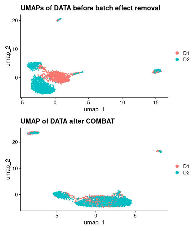
In this step, we can see that the dataset were normalized first using Seurat and then further normalized using COMBAT. And then, Suerat Scaledata is used again, based on the pre-selected HVG.
Very interestingly, the example data is already very well merged at this point. So it is not very clear how one can demonstrate the use of BEER.

print('Calculating PCs ...')
pbmc <- RunPCA(object = pbmc, seed.use=SEED, npcs=PCNUM, features = VariableFeatures(object = pbmc), ndims.print=1,nfeatures.print=1)
 ### make 50 PC pca ###
pbmc <- RunUMAP(pbmc, dims = 1:PCNUM,seed.use = SEED,n.components=N)
for(this_batch in UBATCH){
    this_index=which(BATCH==this_batch)
    this_one=DR[this_index,]
    #CNUM=max(c(5, round(length(this_index)/GNUM) ))
    this_gnum=min(GNUM, (length(this_index)-1))
    this_group=.getGroup(this_one,this_batch,this_gnum)
    #### .getGROUP =  function to perform kmeans clustering of GNUM (30 by default) cluster ###
    GROUP[this_index]=this_group
}
pbmc@meta.data$group=GROUP
VP=.getVPall(pbmc, ROUND)
Using the .getGroup function, each batch was clustered to 30 clusters. Next, using the .getVPall function, 1-to-1 mapping of cluster representative were performed between 2 batches. This is the novel part of BEER and thus lets have a closer look into the code
#.getVPall<- function(pbmc, ROUND){
  print('Finding MN pairs...')
  ################
  #REF=.generate_agg(pbmc@assays$RNA$data, pbmc@meta.data$group)
  exp_sc_mat<-pbmc@assays$RNA$data
  TAG<-pbmc@meta.data$group
  REF=.generate_agg(pbmc@assays$RNA$data, pbmc@meta.data$group)
  ##### breaksdown of the function .generate_agg ###
  ##### so here, for each cluster, mean expression (row mean) were calculated. ####
  #### this generate a representative per cluster ###
  .generate_agg <- function(exp_sc_mat, TAG, print_step=100){
    print_step=100
    NewRef=matrix(0,ncol=length(unique(TAG)),nrow=nrow(exp_sc_mat))
    ### NewRef 6695 x 60 new representative exp matrix
    TAG=as.character(TAG)
    refnames=unique(TAG)
    total_num=length(refnames)
    outnames=c()
    i=1
    #### take exp mean for each cluster for each gene to generate representative
    while(i<=length(refnames)){
      one=refnames[i]
      this_col=which(TAG==one)
      outnames=c(outnames,one)
      if(length(this_col) >1){
        #this_new_ref=apply(exp_sc_mat[,this_col],1,mean)
        this_new_ref=apply(exp_sc_mat[,this_col],1,sum)
      }else{
        this_new_ref = exp_sc_mat[,this_col]
      }
      NewRef[,i]=this_new_ref
      if(i%%print_step==1){print(paste0(i,' / ' ,total_num ))}
      i=i+1
    }
    rownames(NewRef)=rownames(exp_sc_mat)
    colnames(NewRef)=outnames
    if(length(NewRef[1,])==1){
      NewRef=cbind(NewRef[,1], NewRef[,1])
      rownames(NewRef)=rownames(exp_sc_mat)
      colnames(NewRef)=c(outnames,outnames)
    }
    return(NewRef)
  }
#.getVPall cont.
VREF=NewRef
CORMETHOD='spearman'

CVREF=cor(VREF,method=CORMETHOD)
orig.CVREF=CVREF

UBATCH=unique(pbmc@meta.data$batch)
#### UBATCH - "D1" and "D2"
    .get_batch<-function(x){
      y=unlist(strsplit(x,'_'))[1]
      return(y)
    }
    group_batch=apply(as.matrix(colnames(CVREF)),1,.get_batch)

.getMN <- function(this_cor_mat){
      VP=c()
      i=1
      while(i<=nrow(this_cor_mat)){
        this_p1=rownames(this_cor_mat)[i]
        j=1
        while(j<=ncol(this_cor_mat)){
          this_p2=colnames(this_cor_mat)[j]
          this_cor=this_cor_mat[i,j]
          if( this_cor!= -99999  & this_cor==max(this_cor_mat[i,]) & this_cor==max(this_cor_mat[,j])){
            ### so not only b1 has to be the max correlated with b2, b2 also has to be the max correlated with b1
            VP=cbind(VP,c(this_p1,this_p2))
          }
          j=j+1}
        i=i+1}
      return(VP)

    }


    VP=c()
    I=1
    i=1
    while(i<length(UBATCH)){
     j=i+1
        while(j<=length(UBATCH)){
          b1=UBATCH[i]
          b2=UBATCH[j]
          b1i=which(group_batch==b1)
          b2i=which(group_batch==b2)
          this_cor_mat=CVREF[b1i,b2i]
          ### make the correlation matrix fot batch 1 vs batch 2 ###
          this_vp=.getMN(this_cor_mat)
          VP=cbind(VP,this_vp)

          ########################

          ########################
          j=j+1}
        i=i+1
      }

      ########################

      ########################
      print('ROUND:')
      print(I)
      I=I+1
    }


    VP=t(VP)
    VP=unique(VP)
    #######################

    print('Number of MN pairs:')
    print(nrow(VP))
    return(VP)
  }

#> VP
#       [,1]    [,2]
#[1,] "D1_26" "D2_23"
#[2,] "D1_27" "D2_27"
#[3,] "D1_23" "D2_10"
#[4,] "D1_14" "D2_28"
#[5,] "D1_11" "D2_11"
#[6,] "D1_29" "D2_22"
The .getVPall function consist of 2 main sub-functions. .generate_agg would isolated cells (columns) involved with the same cluster and compute the mean of each gene expression value to create the cluster center representative. .getMN function computed the correlation matrix of all cluster representative and identify if a cluster contain a 1-to-1 mapping between batches. The 1-to-1 mapping is defined by the cluster has the highest correlation with its counterpart while the counterpart also has the highest correlation with such cluster. For example, if the counterpart cluster has a higher correlation with another cluster, then MN pair was not established. In this demo dataset, we found 6 1-to-1 mappings between the 2 batches (1 batch contain 30 clusters).
Then we moved on the step to identify and remove the PCs that contain substantial batch effects.
 DR=pbmc@reductions$pca@cell.embeddings

  MAP=rep('NA',length(GROUP))
  MAP[which(GROUP %in% VP[,1])]='V1'
  MAP[which(GROUP %in% VP[,2])]='V2'
  pbmc@meta.data$map=MAP

  OUT=.evaluateProBEER(DR, GROUP, VP)
  ###.evaluateProBEER <- function(DR, GROUP, VP){
    OUT=list()
    VALID_PAIR=VP
    ALL_COR=c()
    ALL_PV=c()
    ALL_LCOR=c()
    ALL_LPV=c()
    ALL_LC1=c()
    ALL_LC2=c()
    print('Evaluating PCs ...')
    print('Start')
    THIS_DR=1
    while(THIS_DR<=ncol(DR)){
      THIS_PC = DR[,THIS_DR]
      lst1_quantile=c()
      lst2_quantile=c()
      i=1
      while(i<=nrow(VALID_PAIR)){
        this_pair=VALID_PAIR[i,]
        this_index1=which(GROUP %in% this_pair[1])
        this_index2=which(GROUP %in% this_pair[2])
        lst1_quantile=c(lst1_quantile,quantile(DR[this_index1,THIS_DR]))
        lst2_quantile=c(lst2_quantile,quantile(DR[this_index2,THIS_DR]))
        i=i+1}

      this_test=cor.test(lst1_quantile, lst2_quantile, method=CORMETHOD)
      ### why are they doing cor.test on quantile values?
      this_cor=this_test$estimate
      this_pv=this_test$p.value

      this_test2=cor.test(lst1_quantile, lst2_quantile, method='pearson')
      this_cor2=this_test2$estimate
      this_pv2=this_test2$p.value

      olddata=data.frame(lst1=lst1_quantile, lst2=lst2_quantile)
      fit=lm(lst1 ~lst2, data=olddata)

      ALL_LC1=c(ALL_LC1, summary(fit)$coefficients[1,4])
      ALL_LC2=c(ALL_LC2, summary(fit)$coefficients[2,4])
      ALL_COR=c(ALL_COR, this_cor)
      ALL_PV=c(ALL_PV, this_pv)
      ALL_LCOR=c(ALL_LCOR, this_cor2)
      ALL_LPV=c(ALL_LPV, this_pv2)
      print(THIS_DR)
      THIS_DR=THIS_DR+1}


    OUT$cor=ALL_COR
    OUT$pv=ALL_PV
    OUT$fdr=p.adjust(ALL_PV,method='fdr')
    OUT$lc1=ALL_LC1
    OUT$lc2=ALL_LC2
    OUT$lcor=ALL_LCOR
    OUT$lpv=ALL_LPV
    OUT$lfdr=p.adjust(ALL_LPV,method='fdr')

    print('Finished!!!')
    return(OUT)
  }
Here, the .evaluateProBEER funtion is for computing the PC values between the 1-to-1 mapping groups. Briefly, from the previously identified MN pair (ie. “D1_26” and “D2_23”), the original PCA cells loadings were recalled (N cells x 50 PC) and isolated based on the cluster assignation. Then, the quantiles of the PC vlaues were obtained for each group and cor.test were performed on the quantile values. I think the quantiles values were taken so as to resolved the issue with different cluster size and so each 1-to-1 cluster pair will have 5 pairs of points (0, 25, 50, 75, 100%) in the cor.test. In here, we have 5 pairs of points x 6 MN pair, thus 30 data points for cor.test for each PC. Finally, cor.test results of each PC is recorded and returned.
### BEER function cont
### writing results
  RESULT=list()
  RESULT$seurat=pbmc
  RESULT$vp=VP
  #RESULT$vpcor=VP_OUT$cor
  RESULT$cor=OUT$cor
  RESULT$pv=OUT$pv
  RESULT$fdr=OUT$fdr
  RESULT$lcor=OUT$lcor
  RESULT$lpv=OUT$lpv
  RESULT$lc1=OUT$lc1
  RESULT$lc2=OUT$lc2
  RESULT$lfdr=OUT$lfdr

  ################
  RESULT$ROUND=ROUND
  RESULT$COMBAT=COMBAT
  RESULT$COMBAT.EXP=COMBAT.EXP
  RESULT$RMG=RMG
  RESULT$GNUM=GNUM
  RESULT$GN=GN
  RESULT$PCNUM=PCNUM
  RESULT$SEED=SEED
  RESULT$N=N
  RESULT$APP='BEER'
  ###############


  PCUSE=which( (rank(RESULT$cor)>=length(RESULT$cor)/2 | RESULT$cor>0.7 )    &
                 (rank(RESULT$lcor) >=length(RESULT$cor)/2 | RESULT$lcor>0.7)   #&
               #p.adjust(RESULT$lc1,method='fdr') >0.05
  )
  ### so select pc with cor >0.7 or above average ###
  RESULT$select=PCUSE

  print('############################################################################')
  print('BEER cheers !!! All main steps finished.')
  print('############################################################################')
  print(Sys.time())

  return(RESULT)
}
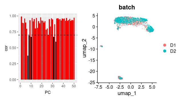
In the final step of BEER, we can see that PC with correlation > 0.7 or correlation values above average PC in the tests were selected. Then UMAP is constructed using Seurat on the COMBAT-normalized combined dataset again, based on the selected PCs by BEER.

Conclusion
So after digging into the codes, I can see that:
1) BEER does use COMBAT and then further remove batch effects based on the PCA.
2) clusters mapping is 1-to-1 and we have to accept that only a small fraction of cells have MN-pair clusters.
3) In this example the batch effect do not affect many PCs after COMBAT correction, so it seems working. The article did present a more drastic case that COMBAT did not work at all. It would be interesting to see which PC they remove to get the merge successful.
4) Finally, there were no further instructions on DE analysis after merging. So I guess we will have the perform biomarker identification individually first to identify biomarker and compare and contrast between batches of cells identified to be in the same cluster in the merged dataset.