Finding the transitional regulation through cell-state density

Mellon Otto et al is a very creative tool to analyse single cell data. The analysis begins with a curated dataset that already have the cell type and clusters defined. Mellon then computes a cell state density of each cell based on the clustering landscape; thus, highlighting regions that are less/more densely populated (edges of the clusters vs center of the clusters) within a cluster. Rather than a rigid cluster boundary, mellon describes the cell-cell relationship in the expression manifold in a continuous manner.

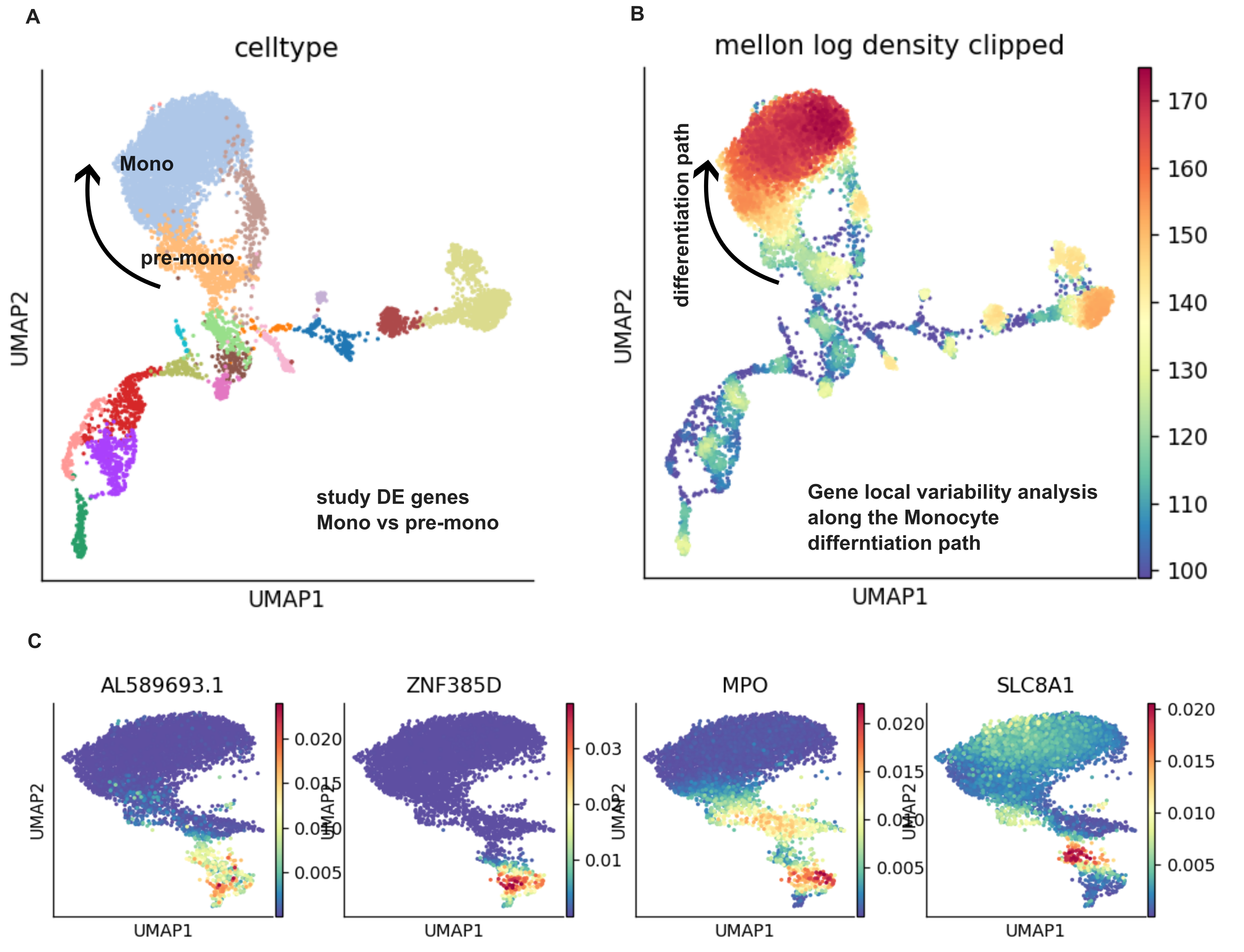
The motivation of studying the location of cells in the lower-representation manifold (i.e PCA axis) is that the low density region may indicate rapid expression changes in a cluster, manifesting a transtional state in differentiation. Instead of comparing the log2fold change between two clusters with manually defined starting and endpoint of differentiation, we can track the gene changes along the “transitional” cells between 2 dense populations that are the sinks (i.e. differentiation end points) of various phenotypes.

A. Umap of the depleted T cells dataset, coloured by cell types. B. Umap coloured by Mellon cell state density. To identify key differentiation changes from pre-monocytes to monocytes, one can calculate differential expression between the 2 clusters. Instead, Mellon investigate the cell state density and look for genes that has the highest local variabilities to search for master regulator involved in the differentiation path. C. Top 4 genes showing the highest local variability in monocyte differentiation identified by Mellon.

Mellon methodology

Mellon builds a diffusion map based on nearest-neighbor distance matrix. It begins with a PCA representation of the scRNA-seq expression matrix (using the top 2500 highly variable genes, using scanpy codes). Then, the cell-cell distance (euclidean) were computed based on the PCA (20 by default).

Meanwhile, GP process were used to fit the diffusion map representation of cells to the assigned cluster nominated by the PCA NN clustering. Here, the 20 DM_EigenVectors were fit to assign cells to 20 cluster, and then the probability density of each cell belonging to the assigned cluster were computed as cell-state density. This again highlight the paramount importance of PCA in single cell datasets, and why we need to choose carefully the number of principal components used in downstream analyses.

In the density landscape described by Mellon, one can identify low density regions (as transitional state with rapid expression changes) between 2 high density clusters (cells in stable states). Gene with high local variability in the low-density regions that "”likely drive fate specifications”“ were ranked based on expression changes (from imputed gene expression by MAGIC) difference from nearest neighbors (default set to 15, determined in umaps) normalised by nearest neighbor distances (default: euclidean distance in the first 20 PC in PCA).

Further gene change variability analyses at shorter differentiation path (i.e cell specialization) vs longer path (stem cell differentiation programs) could help to identify general and lineage specific cell fate regulators.

The code and tutorial

import numpy as np
import matplotlib
import matplotlib.pyplot as plt
from sklearn.cluster import k_means
import palantir
import mellon
import scanpy as sc
import warnings
from numba.core.errors import NumbaDeprecationWarning
warnings.simplefilter("ignore", category=NumbaDeprecationWarning)
matplotlib.rcParams["figure.figsize"] = [4, 4]
matplotlib.rcParams["figure.dpi"] = 125
matplotlib.rcParams["image.cmap"] = "Spectral_r"
# no bounding boxes or axis:
matplotlib.rcParams["axes.spines.bottom"] = "on"
matplotlib.rcParams["axes.spines.top"] = "off"
matplotlib.rcParams["axes.spines.left"] = "on"
matplotlib.rcParams["axes.spines.right"] = "off"
ad = sc.read("data/preprocessed_t-cell-depleted-bm-rna.h5ad")

So Mellon is highly dependent on scanpy and palantir that scanpy would take care of the basic processing the palantir would be used for pseudotime inference and gene variability analysis. And we will use the preprocessed t-cell-depleted bone marrow dataset (GSE200046) in the tutorial. The expression matrix contain 8627 cells x 17226 genes.

ad.obsm["X_pca"]
### 8627 cells x 50 pc 
### build diffusion map using Palantir based on X_pca (generated feom scanpy)
dm_res = palantir.utils.run_diffusion_maps(ad, pca_key="X_pca", n_components=20)
dm_res
### 'T' = 8627x8627 sparse matrix
### 'EigenVectors' = 8627 rows x 20 columns 
### 'EigenValues' = 20 row x 1 Eigenvalue 

In this step, the first 20 PC were used to build a diffusion map and yield the 8627 cells x 20 columns “EigenVectors” representation.

### build Cell density using Mellon
model = mellon.DensityEstimator()
### GP model ###
log_density = model.fit_predict(ad.obsm["DM_EigenVectors"])
predictor = model.predict
predictor:
#A predictor of class "LandmarksConditionalCholesky" with covariance function "Matern52(ls=0.008487226875359388)" trained on 8,627 observations with 20 features and data:
#mu: 88.0053844551665
#jitter: 1e-06
#landmarks: <array 5,000 x 20, dtype=float64>
#weights: <array 5,000, dtype=float64>
# The melln log predictors were present already in the preprocess data #
ad.obs["mellon_log_density"] = log_density
ad.obs["mellon_log_density_clipped"] = np.clip(
    log_density, *np.quantile(log_density, [0.05, 1])
)

Here, Mellon used the “DM_EigenVectors” to fit the GP model to the data and return the log_density of each training point. The model has restricted to learn from 5000 cells each with < 50 features.

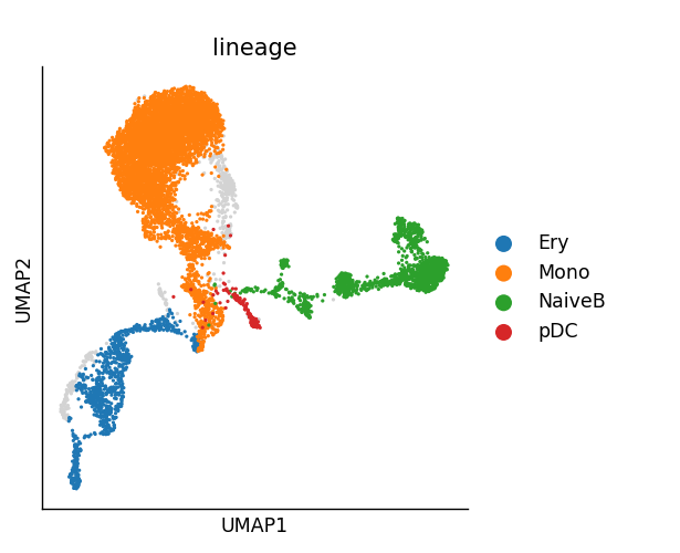
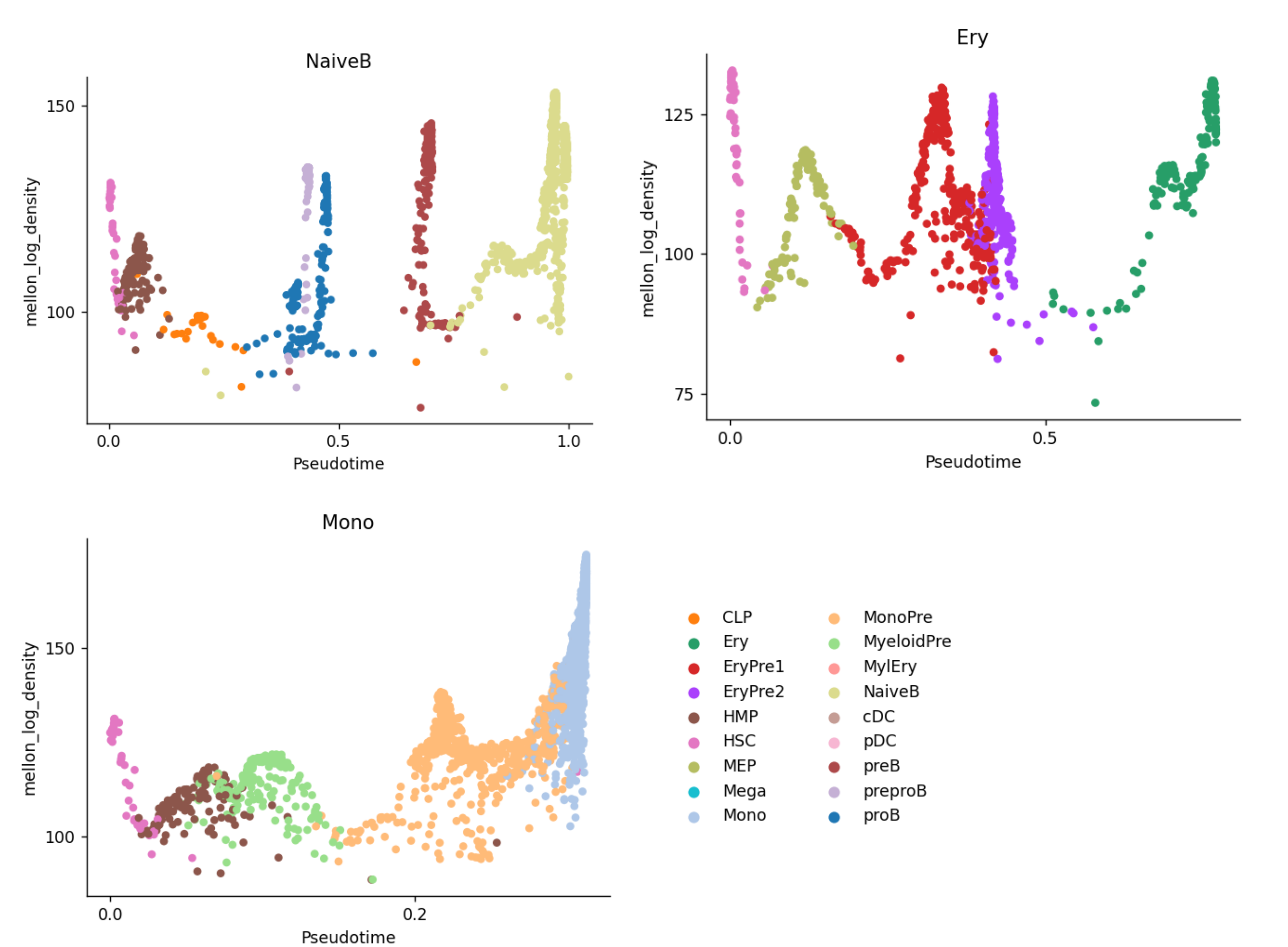
Next, Mellon compared the cell state density along the palantir pseudotime trajectory. There are 4 predefined lineages: NaiveB, Ery, pDC, and Mono present in the dataset, stored at ad.obsm[“palantir_lineage_cells”]. Our aim is to identify genes with high local variability along these lineages. Here, I plotted 3 of the lineages to visualise the cell type and log density distribution.

Umap with cells coloured by palantir pseudotime lineages.

Log_density vs palantir pseudotime lineages.

### Local variability analysis ###
palantir.utils.run_local_variability(ad)
#### take in 'MAGIC_imputed_data', 'distances' and compute the expression variability among neighbors.
### return "local_variability" in .layers
>>>ad.uns['neighbors']
{'connectivities_key': 'connectivities', 'distances_key': 'distances', 'params': {'method': 'umap', 'metric': 'euclidean', 'n_neighbors': 15, 'random_state': 0}}

def _local_var_helper(expressions, distances, eps=1e-16):
    if hasattr(expressions, "todense"):

        def cast(x):
            return x.todense()

        issparse = True
    else:

        def cast(x):
            return x

        issparse = False
    for cell in range(expressions.shape[0]):
        neighbors = distances.getrow(cell).indices if issparse else slice(None)
        try:
            neighbor_expression = cast(expressions[neighbors, :])
            cell_expression = cast(expressions[cell, :])
            expr_deltas = np.array(neighbor_expression - cell_expression)
        except ValueError:
            raise ValueError(f"This cell caused the error: {cell}")
        expr_distance = np.sqrt(np.sum(expr_deltas**2, axis=1, keepdims=True))
        change_rate = expr_deltas / (expr_distance + eps)
        yield np.max(change_rate**2, axis=0)

The _local_var_helper function in palantir is used for calculating local variability of a gene per cell. We can see that it is based on the ‘distances’ computed between the focal cell and its neighbors. More info is stored in ad.uns[‘neighbors’], where specified that the number of nearest neighbor was set to 15. For each cell, the expression difference of a gene between its 15 neighbors were calculated (expr_deltas) normalised by the “expr_distance”; and the max change_rate is reported as the local gene variability of the cell.

### Compute gene score 
score_key = "change_scores"
palantir.utils.run_low_density_variability(
    ad,
    cell_mask="branch_masks",
    density_key="mellon_log_density_clipped",
    score_key=score_key,
)

#>>> ad.layers['local_variability'].shape
#(8627, 17226)
# The function take the local_variability based on cells belonged to a branch, variability values of n cells
# gene score (normalised by density)) = mean(variability values of n cells * np.exp(-ad.obs["mellon_log_density_clipped"].values))
# here higher the density, lower the np.exp value; thus give more weights on the variability observed in low density cells 
### cell_masks = Cell grouping in ad.obsm  
### output: gene scores stored at ad.var 'change_scores_Mono', 'change_scores_pDC', 'change_scores_NaiveB', 'change_scores_Ery'

ad.var['change_scores_Mono'].sort_values(ascending=False)
#AL589693.1    6.388634e-48
#ZNF385D       6.365719e-48
#MPO           5.490143e-48
#SLC8A1        5.289105e-48
#PDE4D         4.801543e-48

And finally, we will compute lineage specific gene local variability by providing the “branch_masks” (palantir lineage map: boolean matrix of whether a cell belongs to a particular lineage). “We next compute, a low-density change score s_jsub> for each gene j, as the sum of the gene-change rates dⁱ_j across the selected cells, inversely weighted by the cell-state densities, ρ(x_i)”:

\[\sum \frac{d_{j}^{i}}{p(x_{i})}\]

We can see that if a gene has high local expression change in many low cell-density cells, the gene change score will be very high. We can then rank gene importance in the cell fate transition by its gene change score.

Conclusion

I like that Mellon show a new dimension of how to interpret the single cell data and a new way to identify key regulators that would experience rapid expression changes to direct cell fate.

However, I can also see that the prerequisite to run Mellon is a set of clean and well-defined dataset. It can be a difficult task to clean up and generate such dataset in the first place, but it will be very rewarding to study them in depth and learn new things from the data afterwards.