Cross-species cell phylogeny construction

Mah and Dunn’s paper developed another way to perform inter-species comparative analyses using single cell datasets. The authors attempted to looked into how eye differentiation may differ/preserved across five species by comparing cluster specific marker genes. Rather than performing the clustering and cell type identification of each species sample individually and then perform comparative analysis between clusters of the same cell type, the authors here built a cell phylogeny tree from an integrated datasets of all species and then perform cluster extraction.
The cell phylogeny constructed identified gene sets that were “ancestral”, driving the differentiation in all species investigated, underpinning the basic blueprint for eye construction.

I think the authors have proposed a very interesting methods to perform comparative analyse in scRNA-seq datasets and have set up a banchmark for cleaning and integrating data. Therefore, I spent more time to work out why than how in studying their code. They also have a very clear documentation in github and I do appreciated how easy it was to dollow their analyses.

Step 1 + 2 cleaning and integrating the datasets

THe authors reanalysed the datasets from Zyl et al (2020) that performed scRNA-seq on the eyes of 5 model organisms.

The cleaning and integration of the 5 datasets were found in 1_Wrangle_Data.Rmd and 2_Create_Matrices.Rmd. The phylogenetic analysis started at 3_PC_sweep_analysis.Rmd and we will started there.

Step 3 building cell PCA.

Step 3 commenced with a integrated cell matrix of 919 cells. Each cell type of a species has 10 cells and each species has 15-20 cell types. The 10 cell were randomly sampled from the raw scRNA-seq datasets based on annotations from Zyl et al.

#perform PCA on the cross-species integrated matrix.
make_pc_sweep_infiles(matrix_path="~/cellphylo/analysis/matrix/cross-species_integration/aqhumor_cross_species_integrated_mtx/", run_PCA=TRUE, PC_range=c(3:10))
### mat: 2000 gene features x 919 cells 
### use pylip contml to make a tree for each PC-sweep file

Here, the make_pc_sweep_infiles function took in a gene x cell matrix, transpose it and then performed PCA on it. The resultant pc$x has the 919 cells x 919 PC loadings. Each pc$x PC were centered and normalized to unit vector and then used as input columns as pylip contml that use continuous features (as columns) to build trees.

One can think of the pc$x recorded each cell’s weight on each of the 919 PC. In other words, one can use the PCA to identify which cell looks best as a “model” cell for a particular group. And cells with similar gene expressions would be close to each other in a cell PC. According to the authors these PC had filtered out the most salient cell-type signals for contml tree construction.

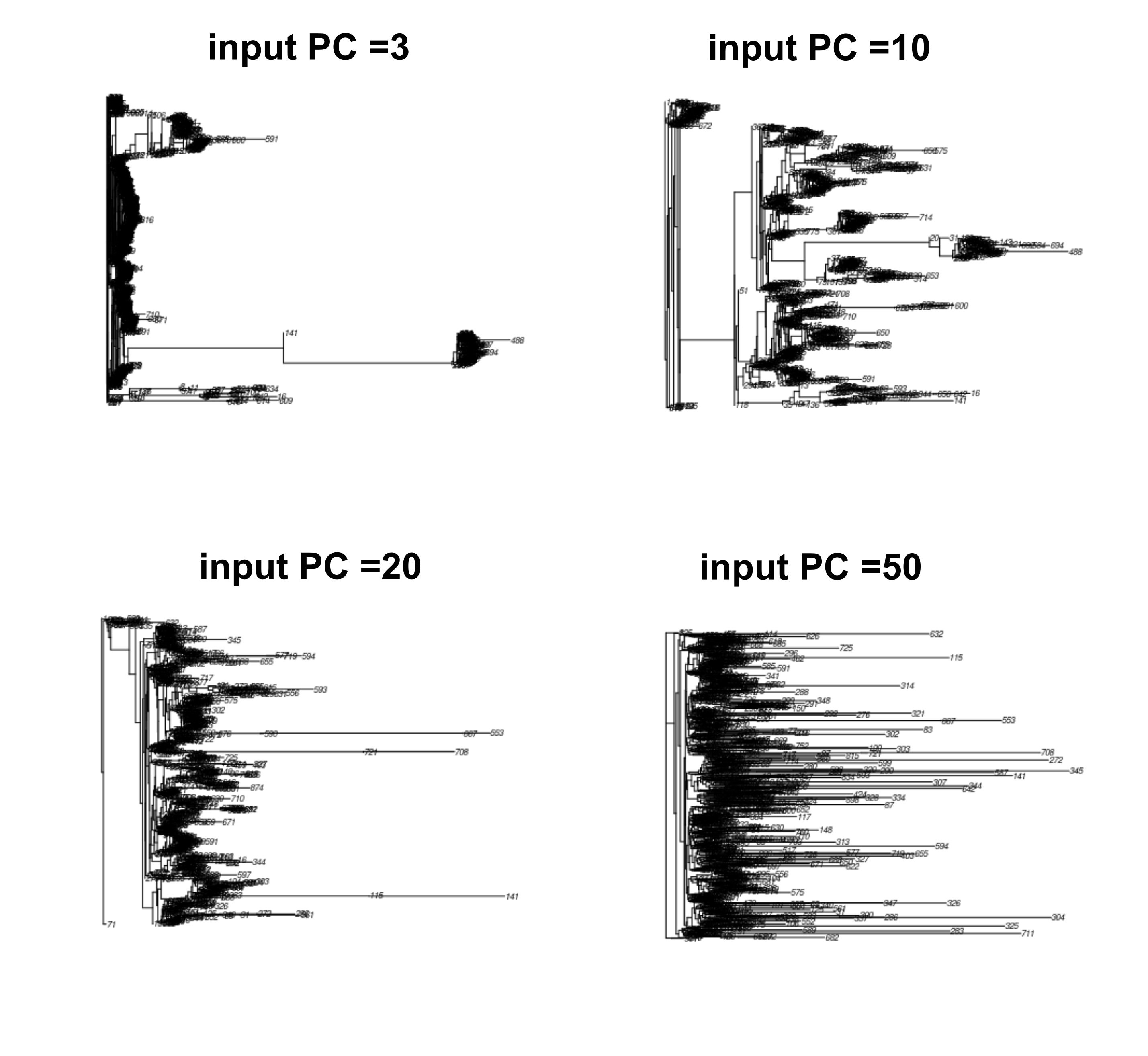
The PC_sweep, generate input matrix of 3 to 100 PCs for contml constructions. One can perceived that these PC present a “model” cell type, so if there were too few PC, cells types would not be well resolved, but if too many PCs were put in, cells were split too much in the trees and all common signals would be lost.

And we can see that in the output tree, the tip got longer as more PC were used for the input for Phylip.

Contml output trees with different numbers of input PCs.

The authors settled that 20PC are the best option, as stated in the article. It is consistent with the initial experimental design that 15-20 cells types were selected for each species in the input file.

4_Jumble_analysis.Rmd

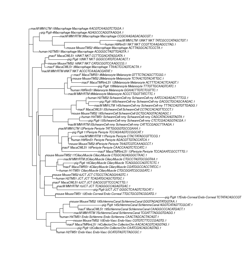
After settling on 20 PCs, the authors further filtered the cell list to 54 cells input (1 cell per cell type per species) to identify the best tree using Jumble score. This resemble to build tree with 1 orthologus gene sequence from each species, each species have 10 paralogues. We can expect the tree would have 10 branches reflecting the 10 paralogus group and under each paralogue clade, we would have the tips of orthologues from each species.

The authors provided the jumble trees output for reproducibility and we used those output to continue the analyses.

#path to contml outtrees (empty files removed)
tree_dir_path = "jumble/output/outtrees_54_jumble_search_processed/"

#find best jumble tree
best_jumble_tree(tree_dir_path = tree_dir_path)
list.files(tree_dir_path)

#### best_jumble_tree in cellphylo_functions. R###
best_jumble_tree <- function(tree_dir_path, multiphylo){
scored_trees <- lapply(trees, function(trees){
    focal_tree_path <- trees
    output <- score_jumble(multiphylo = multiphylo,focal_tree_obj = trees, print=FALSE )
    return(output)
  }) #function close, lapply close
  
  
  #max sum of jumble scores
  jumble_sums <- lapply(scored_trees, function(scored_trees){
    sums <- scored_trees$score_sum
  })
  index = which(jumble_sums == max(unlist(jumble_sums)))
  print(paste0("max sum of scores =  index: " , index, " score: ", max(unlist(jumble_sums))))
 }

score_jumble <- function(multiphylo, focal_tree_path, focal_tree_obj, print){
  #multiphylo file
  jumble_trees <- multiphylo
 #calculate jackknife scores
  scored_tree <- plotBS(main_tree, jumble_trees, type="none", bs.col="red", method = "FBP")
    if (print==TRUE){
    #for soem reason figtree does not display tree if not midpoint-rooted. ape::write.tree still prints correctly even if unrooted. midpoint() before writing
    #print out tree
    ape::write.tree(scored_tree, file="scored_tree.tre")
  }

So the authors performed dozens times of contml to get a collections of tree, then use the plotBS function to score each tree’s bootstrap values based on all the contml output trees. The plotBS function returns a bootstrap value for each node of the tree to indicate the robustness of that node’s presence in the trees (1-100, 100 means the nodes is always present, thus high confidence).

The jumble score of a tree is the sum of all node bootstrap values; and the authors use the jumble scores to identify the best tree.

Similar procedures were carried out to produce the best jackknife trees.

6_Average_cells.Rmd and 7_GO_and_phenetic_trees.Rmd

Step 6 is an interesting concept of constructing a “average” cell in the 20 PCs for a cell types and used these “average” cells to make a tree.

#Input matrix
#919 cells - 10 cells per cell type cluster, 92 cell type cluster
# make 54 cell average cells phylip input 
mat <- Read10X("~/cellphylo/analysis/scjackknife/contml_919cell_subset_20PC_mtx/")
### matrix of 919 cells x 20 PCs
mat <- t(as.matrix(mat))

#limit the cells to the 54 cell type groups
permissible_cells <- read.table("~/cellphylo/analysis/scjackknife/540_cell_subset_cell_ids.txt") %>% unlist()
mat.filtered <- mat[,which(colnames(mat) %in% permissible_cells)]

#parse out annotations
orig_ids <- colnames(mat.filtered)
species <- sapply(strsplit(orig_ids, "_"), function(v){return(v[1])})
cluster_id <- sapply(strsplit(orig_ids, "_"), function(v){return(v[3])})
cell_type_id <- sapply(strsplit(orig_ids, "_"), function(v){return(v[4])})
species_cluster <- paste0(species, "_", cluster_id)
#54 species cluster ids
unique.species_cluster <- unique(species_cluster)

means <- sapply(1:length(unique.species_cluster), function(i){
    mat.subset <- mat.filtered[,which(species_cluster == unique.species_cluster[i])]
  means.df <- rowMeans(mat.subset) %>% as.data.frame()
  colnames(means.df) <- unique.species_cluster[i]
    return(means.df)
  }) #close apply

means_mat <- as.data.frame(means)
## Create infile for contml

Step 7 is the most exciting part. After conferring a confident 54 cell phylogeny, we can proceed to use the first 20PC of the 919 cells to identify biomarkers. We went back to the 919 cells pc$x.

#load matrix 
#this matrix file was created for the GO analysis. However, it corresponds to the PCA matrix of Fig. S1 step 7
pca <- readRDS("/media/achu/新增磁碟區/cellphylo/analysis/GO_enrichment/PCA_919x919_matrix.rds")

#extract loading values
#pca$rotation are the gene loadings for each pc
### pca$rotation== 2000 genes x 919 cells ###
loadings <- pca$rotation %>% as.data.frame()

#extract loading values
#pca$rotation are the gene loadings for each pc
loadings <- pca$rotation %>% as.data.frame()

#prepare loadings dataframe for lapply function
loadings <- rownames_to_column(loadings, var="gene_symbol")
#index for lapply function. First column of loadings is not a PC
n_pc <- 1:(ncol(loadings)-1)

#order each PC by most positive and most negative gene loadings
order  <- lapply(n_pc, function(pc_index){
  #name of PC column are we working iwth
  PCn <- paste0("PC", pc_index)
  #isolate gene symbol column and PC column
  pc_column <- loadings[,c("gene_symbol", PCn)]
  # "-" sorts by descending (highest value first)
  by_most_pos <- pc_column[order(-pc_column[,2]),] %>% dplyr::select(gene_symbol)
  colnames(by_most_pos) <- PCn
  by_most_neg <-  pc_column[order(pc_column[,2]),] %>% dplyr::select(gene_symbol)
  colnames(by_most_neg) <- PCn
  
  output <- list("positive" = by_most_pos, "negative" = by_most_neg)
  
  return(output)
})
positive <- sapply(order, "[[", "positive")
positive_df <- do.call(cbind, positive)
positive_df <- as.data.frame(positive_df) #a data frame listing the most positively loaded genes, in descending value, for each PC

negative <- sapply(order, "[[", "negative")
negative_df <- do.call(cbind, negative) 
negative_df <- as.data.frame(negative_df) #a data frame listing the most negatively loaded genes, in ascending order, for each PC

The positive_df listed the most positively loaded gene in each PC and vice versa the negative_df listed the most negatively loaded genes in each PC. And finally, the authors performed GO enrichment on the first 20PC with the most 100 +ve/-ve loaded gene per PC. This is a very interesting way to identify DEGs and seems to share some similarity with the concepts of weighted gene co-expression network analysis (WGCNA).

Conclusion

I really enjoyed reading this paper and going through their analysis. The concept provided me a new way to look at single cell data and deepened my understandings of PCA. It is very cool that we can utilize PCA to somewhat generate a “average” cell (center of the cluster) and it is actually emitted meaningful biomarker signals that define the key differentiation events across species. I wonder if these could help us to identify differentiation key regulators using this method.

Anyhow, i think the method were made possible because of the correct integrations and cleaning of multiple raw scRNA-seq datasets. It would be interesting to see if we can get the same results if other integrations methods were implemented.