‘factorize-recover’ perturb-seq.

This is a newer method to infer gene-regulatory network from pooled CRISPR screens with the main aim to infer gene perturbation effect.

More specifically, one can infer gene purterbution effects in a pooled CRISPR screen by reading out the scRNA profile or other phenotype such as viability. Meanshile, the perturbations generate many different conditions and each scRNA profile manifest to a perturbed condition and summarizing correlated genes in these many conditions could reveal networks of co-regulated genes. In that light, the search for GRN was a subsequent analysis from a Perturbation analysis.

Here, Yao et al 2023 demonstrated that guide pooled perturb-seq is highly apt for finding large effect genes as well as inferring GRN. The main idea here is to perform high-MOI CIRSPRi screen followed by scRNA-seq (FR-Perturb) to capture perturbation effect on expression changes.
The assumption of a spass effect matrix and additive mutation effect enable the author to summarize both perturbation effects and consequential differential expressions efficiently using only a small number of cells with excite-seq after perturbation.

FR-Perturb code

“FR-Perturb first factorizes the expression count matrix with sparse factorization (that is, sparse principal component analysis (PCA)), followed by sparse recovery (that is, least absolute shrinkage and selection operator (LASSO)) on the resulting left factor matrix comprising perturbation effects on the latent factors. Finally, it computes perturbation effects on individual genes as the product of the left factor matrix from the recovery step with the right factor matrix (comprising gene weights in each latent factor) from the first factorization step (Fig. 1e and Methods).”

This is the description of the FR-Perturb code and let’s have a look in details.

First, I set up the enviroment based on the instructions in FR-perturb github and downloaded the guide pooled perturb seq data (GEO accession: GSM6858450).

import numpy as np
import pandas as pd
import scipy 
import spams
import scanpy
import time, sys, traceback, argparse
import os
import tqdm
import statsmodels.api as sma
import statsmodels.stats as sms
import functools
from tqdm.contrib.concurrent import thread_map

dat = scanpy.read_h5ad("GSM6858450_KD_guide_pooled.h5ad")
### (24192, 15668) 24192 cell x 15668 gene
#>>> dat
#AnnData object with n_obs × n_vars = 24192 × 15668
#    obs: 'Biological_replicate', 'Total_RNA_count', 'Total_unique_genes', 'Percent_mitochondrial_reads', 'Guides', 'Guides_collapsed_by_gene', 'Total_number_of_guides', '10X_channel', 'S_score', 'G2M_score', 'Cell_cycle_phase'
#    var: '_index', 'features'
#>>> dat.X.shape
#(24192, 15668)

p_mat_pd = pd.read_csv("GSM6858450_KD_guide_pooled_perturbations.txt.gz", compression='gzip', index_col = 0, delim_whitespace=True)
### gene x cell table (600 x 24192 cells)

dat.obs.index.equals(p_mat_pd.columns)
#True

The data consisted of 2 objects, 1 is the scRNA-seq .h5ad file and the binary perturbation matrix. The h5ad object contained the expression matrix of 24192 cells x 15668 genes and the meta data of the cells. The perturbation matrix is a 600 gene x 24192 cells matrix.

# center rows of p_mat
### make the total sum of guides_per_cell = 1
guides_per_cell = np.array(p_mat_pd.sum(axis = 0))
p_mat_pd = p_mat_pd.divide(guides_per_cell[np.newaxis, :])
scanpy.pp.normalize_total(dat, target_sum = 10000)
scanpy.pp.log1p(dat)
##Normalize each cell by total counts over all genes, so that every cell has the same total count after normalization.
### calculate log(TP10K+1)
logmeanexp = np.squeeze(np.array(np.log(np.mean(dat.X, axis = 0))))
### return (15668, ) mean gene expression values   
dat.X = dat.X - dat.X.mean(axis = 0)

# center expression matrix based on control expression
n_guides = p_mat_pd.values.sum(axis = 0)
nt_names = ['non-targeting', 'safe-targeting']
### compared dat with paper's table S1
ctrl_idx = np.logical_and(n_guides == 1, p_mat_pd.loc[nt_names].sum(axis = 0).values != 0)
ctrl_exp = dat.X[ctrl_idx,:].mean(axis = 0)
#### removed control basal exp 
#### y'i= log(yi) − log(c)
dat.X = dat.X - ctrl_exp

There the code computes log(transcript per 10K) for the expression matrix “dat.X”, then centered the expression.

lambda1=0.1
rank=20
dat.X = dat.X[:,np.squeeze(np.array(dat.X.sum(axis = 0))) != 0]
keep_cells = p_mat_pd.sum(axis = 0) > 0
p_mat = np.asfortranarray(p_mat_pd.loc[:, keep_cells].T).astype(np.float32)
### p_mat.shape = 24192 x 600 
#### summarize exp into 20 PCA
W = spams.trainDL(np.asfortranarray(dat.X.T), K=rank, lambda1=lambda1, iter=50, verbose=False)
### W.shape=(15668, 20)
U_tilde = spams.lasso(np.asfortranarray(dat.X.T), D=W, lambda1=lambda1, verbose=False)
### dat.X.T = 15668 x 24192
### W = 15668 x 20
### U_tilde = 20x24192 sparse matrix of type '<class 'numpy.float64'
### lasso on expression based on W? 
U_tilde = U_tilde[:, keep_cells]
### cell loading based on the 20 PC (K factor)
U_tilde = np.asfortranarray(U_tilde.T.todense()).astype(np.float32)
### 24192 cells x 20 PC (after translation)
W = W.T
### 20 x 15688 genes

This is the code that perform the sparse principal component analysis (PCA)), followed by LASSO. First, the total PC (rank) was set as 20. After filtering cells without any guide keep_cells = p_mat_pd.sum(axis = 0) > 0, PCA was performed by the function (spams.trainDL).

Next, LASSO was performed and the sparse matrix U_tilde is the cell loading, so called the latent space, on the 20 PC.

#        Regressing left factor matrix on perturbation design matrix...  ')
lambda2=10
U = spams.lasso(U_tilde, D=p_mat, lambda1=lambda2, verbose=False)
### U_tilde = 24192 x 20
### p_mat = 24192 x 600
### U = 600x20 sparse matrix of type '<class 'numpy.float32'>
B = U.dot(W)
### U = 600x20
### W = 20 x 15688
### B = 600 x 15688 perturbation x gene matrix 

LASSO was performed again on U_tilde (24192 cells x 20 PC), given p_mat (24192 cells x 600 perturbation) and return the loading of 600 perturbation on the 20 PC.

And finally, B, the perturbation x gene matrix which indicate the effect of each guide on gene expression is computed.

Interestingly, all the q-values computed in this run did not reach the filtering threshold (q < 0.2).

Perturbations analyses

So, Here we looked into the downstream analyses after obtaining the gene effect x perturbation matrix.
First, we followed the paper instructions to cluster genes that show similar DE patterns (thus co-regulation) across perturbed conditions.

“First, the Euclidean distance between all pairs of genes was calculated by their perturbation effect sizes, and the FindNeighbors function from the Seurat R package was used to compute a shared nearest neighbor graph from these distances (k=20)”

library(Seurat)
library(tidyverse)
library(ggplot2)
lfc<-read_delim("GSM6858450_LFCs.txt")
L<-lfc %>% gather(perturbation, effect, 2:601)

### step 1 caluclate genes Euclidian distance by their perturbation effect 
x<- lfc[, 2:601]
x<- x[]
x<- as.matrix(x)
colnames(x)<- colnames(lfc)[2:601]
rownames(x)<- lfc$`_index`
d<-dist(x, method = "euclidean")
gene_neigbors<- FindNeighbors(d,  k.param=20,compute.SNN=T)
gene_clusters<- FindClusters(gene_neigbors$snn, resolution = 0.5)
gene_clusters$"_index"<- rownames(gene_clusters)
L<- left_join(L, gene_clusters)
# Number of communities: 8

#### find top 2000 genes based on the average magnitude of effects ####
top_downstreme_genes<-L %>% group_by(`_index`) %>% summarise(avg_effect=mean(abs(effect), na.rm = T)) %>% 
  arrange(desc(avg_effect)) %>% rowid_to_column() %>% filter(rowid<=2000) %>% ungroup %>% select(`_index`) %>% unlist()

L %>% filter(`_index` %in% top_downstreme_genes) %>% 
  ggplot(aes(x=res.0.5, y=effect, group=res.0.5))+ geom_boxplot()+
  labs(x="clusters res=0.5", y="perturbation effects", title="Gene perturbation effects among the\n top downstream genes across perturbations")

Gene clustering based on DE across perturbation conditions.

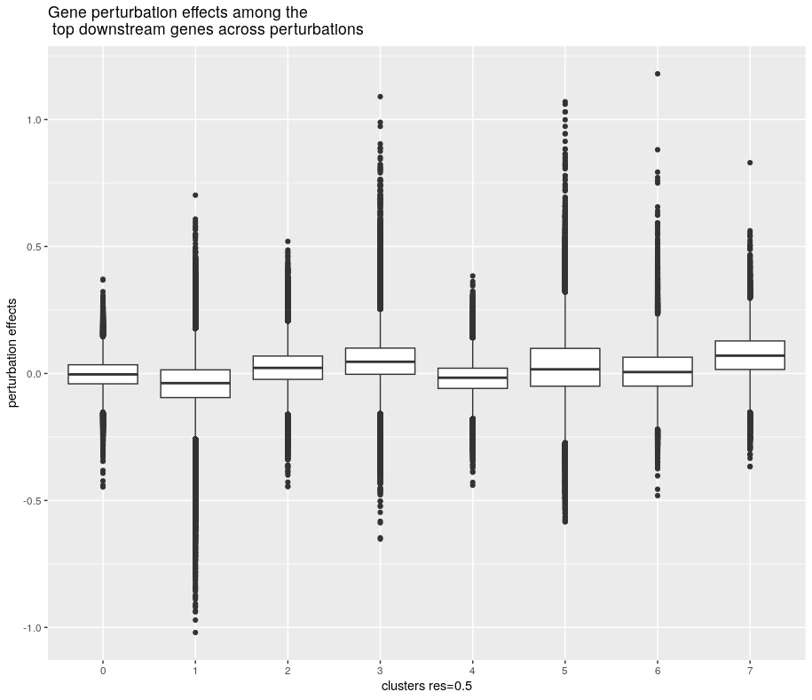
So according to the paper, 4 clustered were manually inspected and selected for gene enrichment analyses using cluster profiler. Top 2000 downstream (perturbed) genes were selected based on average perturbation size. We can see that cluster 1, 3, and contained downstream genes with more extreme perturbation effects.

On another aspect, I am interested in looking to perturbations that generate similar or different effects. It would be the foundation in pairing gene targets that generate orthogonal effects, thus broad coverage, in later combined screens.

Here, I first looked into the top 50 perturbations that altered the highest number of genes. To do so, I filtered out gene with the top and bottom 5% of perturbation effects and quantify the number of extremely perturbed genes in each perturbation. Then, we identified the top 50 perturbation with the most affected genes.

L<-lfc %>% gather(perturbation, effect, 2:601)
L %>% filter(`_index` == perturbation) %>% ggplot(aes(x=effect)) + geom_histogram()
### ook for high perturbingin genes
quantile(L$effect,probs = c(0.05, 0.95))
top_perturbation_genes<-L %>% filter(effect< -0.144 | effect > 0.159) %>%
  group_by(perturbation) %>% summarise(n=n()) %>% arrange(desc(n)) %>% rowid_to_column() %>% filter(rowid<=50)

#### cluster perturbations to see which perturbation generate similar effects ###
d<-dist(t(x), method = "euclidean")
perturbation_neigbors<- FindNeighbors(d,  k.param=20,compute.SNN=T)
perturbation_clusters<- FindClusters(perturbation_neigbors$snn, resolution = 0.8)
perturbation_clusters$"_index"<- rownames(perturbation_clusters)
# Number of communities: 4

h<-lfc[lfc$`_index` %in% top_downstreme_genes, colnames(lfc) %in% top_perturbation_genes$perturbation]
rownames(h)<-lfc$`_index`[lfc$`_index` %in% top_downstreme_genes]
pheatmap::pheatmap(as.matrix(h), labels_row='')

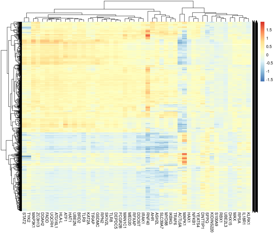
Next, similar to gene clustering to identify co-regulated genes, we also clustered the perturbations. There were 4 clusters found.

Finally, we created a heat map based on the top 2000 perturbed genes and the top 50 perturbation. We can see that the perturbations can be briefly divided into 2 groups and the grouping somewhat were in agreement with Figure 5d;right panel in the paper.

Perturbation effects heat map based on top 2000 perturbed genes x top 50 perturbation condition

Comments

So, we explore the concept and codes of FR-perturb, which infer perturbation effects based on pooled screens. Looking into the code, FR-perturb first summarize DE from scRNA-seq datasets to a 20 dimension latent space. Next FR-perturb summarize perturbation into a 20 dimension latent space. Finally, the dot product of the perturbation x 20 PC . 20PC x gene weight results into the gene x perturbation effect matrix.

The paper’s dataset did not have enough power to generate convincing FDR with the q-values. So we can expect that future experiments will still require more cells in the guide-pooled experiments.

But, it provides a direct way to evaluate gene CRISPR knock-down effects in a high through-put way, and we can see that it will be useful in both GRN inference and future perturb-seq experimental design.