Confidently infer clusters.

So this time I am looking into this paper “Significance analysis for clustering with single-cell RNA-sequencing data”. This study focuses on the issues with the clustering in scRNA-seq pipelines and show an inspiring way to QC whether the clustering is valid or not. Unsupervised clustering based on highly variable genes is a key step in the scRNA-seq pipeline that enables the downstream DE analysis between clusters for finding relevant biomarkers. The defining biomarkers of a cluster are crucial for cell ID, comparative/canonical correlation analyses, etc. for subsequent investigation of the single cell dataset. Therefore, getting the clustering correct is important.

However, the authors in the study found that most ready-to-use packages over-cluster the dataset and were not able to spot the mistakes by typical stability analyses.
The authors found that clustering algorithms “will partition data even in cases where there is only uninteresting random variation present.” The “forcing of a single population into 2 clusters may results in incorrect identification of differences (DE genes with small effect but highly significant p-values)”.

Then, the authors suggest a very nice solution to QC the validity of the clustering by Significance of hierarchical clustering (SHC). In brief, they first perform hclust for the whole dataset. In each split from the root, it calculate the Ward’s linkage between the 2 cluster.

Ward linkage = (ESS(whole population)-(ESS(cluster1)+ESS(cluster2)))/ total number of cells.

The essence of the ward linkage is that if the error sum of squares (ESS) of the cluster mean of whole population is bigger than the sum of ESS of 2 cluster, the split is justified because it minimize the ESS.

However, how big the Ward’s linkage is needed to justify a split? To put a p-value on the empirical Ward’s linkage, a null dataset of 1000 dummy cells is generated from randomly sampling gene expression from a single Poisson log-normal(μ_g, 3) distribution, with μ_g sampled from a Normal(0, 2) distribution). 10 rounds of the null datasets were generated and used to compute the ward linkage after the null data was forced to split into 2 cluster. With the p-value, one can justify the split using a FWER threshold < alpha; in the paper alpha is recommended as 0.25.

This is quite a clever idea and now we can have a look at the code on how they achieve it.

The Code

Actually the codes are valuable to me as I can how see some more math intense packages used such as scry and they are doing things quite differently.

library(scSHC)
library(dendextend)
library(MASS)
data("counts")
counts
dim(counts)
#[1] 32738  1154
# This is a sparse matrix with 32,738 genes and 1,154 cells; the first 577 cells belong to one group, and the second 577 cells to another.
# scSHC
data<-counts
clusters <- scSHC(counts)
clusters[[2]]

         levelName
1 Node 0: 0       
2  ¦--Cluster 1: 1
3  °--Cluster 2: 1

Starting with the demo datasets of scSHC, the program has found that it only has 2 clusters. Now, we will take apart the scSHC function and look into the underlying codes in more details.

### set up scSHC parameter
alpha = 0.05
num_features = 2500
num_PCs = 30
cores <- 
batch <- rep("1", ncol(data))  
batch <- as.character(batch)
attr(batch, "names")<- unlist(data@Dimnames[2])
colnames(data) <- paste0("cell", 1:ncol(data))

### perform pca for 30 PC
dev <- scry::devianceFeatureSelection(data)
### filter HVG up to 2500 genes
var.genes <- rownames(data)[order(dev, decreasing = T)[1:num_features]]
### pca
#gm.x <- reduce_dimension(data[var.genes, ], batch, num_PCs)[[2]]
### reduce_dimension in sc_SHC/utilities.R
y<-data[var.genes, ]
x<- batch
pdev <- poisson_dev_batch(y,x) ### genes x cells matrix 
pdev <- t(scale(Matrix::t(pdev),scale=F))
PCs <- RSpectra::eigs_sym(as.matrix(tcrossprod(pdev)),k=num_PCs)
gm.x <- t(crossprod(PCs$vectors,pdev)) ### 1154 cells x 30 PC 
### gen distance matrix
gm.d <- dist(gm.x)
hcl <- fastcluster::hclust(gm.d, method = "ward.D")
dend <- as.dendrogram(hcl)
dends_to_test <- list(dend)
### a list of binary splits of dendrogram ##

So here is very cool to see the function RSpectra::eigs_sym will directly generate PCA with assigned number of PC. The function “poisson_dev_batch” is the sc-SHC utility function, it calculates the deviation of each gene. gm.x is the loading of each cell in all PC. Then we perform hclust on the distance matrix (gm.d) of gm.x to generate the dendrogram.

Now we are ready to test the split.

clusters <- list()
node0 <- NULL
counter <- 0
parents <- list("root")

### First cut from root ###
cuts <- dendextend::cutree(dends_to_test[[1]], k = 2, order_clusters_as_data = F)
### get group label of tree for this cut ###
leaves <- get_leaves_attr(dends_to_test[[1]], "label")
### get cell names 
ids1 <- leaves[cuts == 1]
ids2 <- leaves[cuts == 2]
### get cells for the 2 group ###
alpha_level <- alpha * ((length(leaves) - 1)/(ncol(data) - 1))
### so the alpha_level becomes smaller and smaller as we do down to each split
tab <- table(batch[c(ids1, ids2)], cuts)
to.keep <- rownames(tab)[which(matrixStats::rowMins(tab) > 20)]
### so batch have to have at least 20 cells ###
ids1 <- ids1[batch[ids1] %in% to.keep]
ids2 <- ids2[batch[ids2] %in% to.keep]

So now we have the cells in 2 groups, split by the “dends_to_test[[1]]”, the first split of the tree.

 test <- test_split(data, ids1, ids2, var.genes, num_PCs, batch, alpha_level, cores, posthoc = F)
### look into test_split function ###
# Re-order data
cell1s <- data[,ids1]
cell2s <- data[,ids2]
true <- cbind(cell1s,cell2s)
batch <- batch[c(ids1,ids2)]

# Re-run dimension reduction and calculate test statistic
gm <- reduce_dimension(true[var.genes,],batch,num_PCs)
gm_sub.x <- gm[[2]]
labs <- c(rep(1,length(ids1)),rep(2,length(ids2)))
### generate a vector labels of the cluster of all cells ###
Qclust <- sapply(unique(batch),function(b) ward_linkage(gm_sub.x[batch==b,],labs[batch==b]))
### compute ward linkage of the 2 cluster ###
stat <- median(Qclust)
#> stat
#[1] 3541.71

So here we have the Ward’s linkage of the 2 cluster. Then we compute the null distribution.

# Determine the set of stable "on" genes
### utilities function of sc-SHC
poisson_dispersion_stats <- function(y){
  n <- Matrix::colSums(y) ### a vector of sum of read of each cell 
  pis <- Matrix::rowSums(y)/sum(y) ### a vector of sum of read of each gene/ total read of matrix? ###
  mu <- crossprod(array(pis,dim=c(1,length(pis))),array(n,dim=c(1,length(n)))) ### reconstruct a gene x cell matrix 
  y2 <- (y - mu)^2 / mu ### compute empirical - expect value of exp , square to make variance ###
  disp <- Matrix::rowSums(y2)/ncol(y2)
  if (!'matrix'%in%class(y2)) {
    y2 <- as.matrix(y2)
  }
  return(sqrt(ncol(y))*(disp-1)/sqrt(matrixStats::rowVars(y2)))
}
phi_stat <- poisson_dispersion_stats(true[var.genes,])

check_means <- matrixStats::rowMins(sapply(unique(batch),function(b) Matrix::rowSums(true[var.genes,batch==b])))
on_genes <- which(pnorm(phi_stat,lower.tail=F)<0.05&check_means!=0)
### pnorm(phi_stat,lower.tail=F)<0.05 check low dispersion genes with large exp mean ###

Now we are now ready to fit the null model.

# Fit model
params <- fit_model(true[var.genes,],on_genes,batch,num_PCs)
### go to fit_model_batch() in clustering.R
function(y,on_genes,num_PCs){
y=true[var.genes,]
# Compute sample moments of the on genes
on_counts <- Matrix::t(y[on_genes,])
cov <- cov(as.matrix(on_counts))
means <- Matrix::colMeans(on_counts)
### build mean and covariance matrix for on_genes ###
# Use method of moments to estimate parameters
sigmas <- log(((diag(cov)-means)/means^2)+1)
mus <- log(means)-0.5*sigmas
mus.sum <- tcrossprod(array(mus,dim=c(length(mus),1)), array(1,dim=c(length(mus),1)))+
           tcrossprod(array(1,dim=c(length(mus),1)),array(mus,dim=c(length(mus),1)))

#p<-tcrossprod(array(mus,dim=c(length(mus),1)), array(1,dim=c(length(mus),1)))
#q<-tcrossprod(array(1,dim=c(length(mus),1)),array(mus,dim=c(length(mus),1)))
# p= 2089 x 2089 matrix that each row has the same value 
# q= 2089 x 2089 matrix that each column has the same value 
sigmas.sum <- tcrossprod(array(sigmas,dim=c(length(sigmas),1)), array(1,dim=c(length(sigmas),1)))+
              tcrossprod(array(1,dim=c(length(sigmas),1)), array(sigmas,dim=c(length(sigmas),1)))

rhos <- suppressWarnings(log(cov/(exp(mus.sum+0.5*sigmas.sum))+1))
rhos[is.na(rhos)|is.infinite(rhos)] <- (-10)
diag(rhos) <- sigmas

# Make the covariance matrix positive-definite
on_cov_eigs <- RSpectra::eigs_sym(as.matrix(rhos),k=min(c(nrow(rhos)-1,num_PCs)))
num_pos <- sum(on_cov_eigs$values>0)
### cut PC that have neg. values ###
on_cov.sub <- on_cov_eigs$vectors[,1:num_pos]%*%sqrt(diag(on_cov_eigs$values[1:num_pos]))
on_cov <- tcrossprod(on_cov.sub)
diag(on_cov) <- diag(rhos)
on_cov <- sfsmisc::posdefify(on_cov)
on_cov.sqrt <- t(chol(on_cov))
## generate all params for fitting poisson distribution later ###
return(list(Matrix::rowMeans(y),mus,on_cov.sqrt))
}

So here fit model return the imputed parameters (mean exp vector, mus(reconstructed exp mean for on_genes), and on_cov.sqrt (covariance matrix of on-genes)) that we need to recontruct the a null data matrix given that all gene expression are sample from 1 single population.

# Generate null distribution of test statistics, iterate for 10 times? 
  Qclusts2_1 <- mclapply(1:10,function(i) {
    generate_null_statistic(true[var.genes,],params,on_genes,batch,
                            num_PCs,gm,labs,posthoc)
  },mc.cores=cores)
### run on multi-score, iterate for 10 times, generate mull stats 

### generate null 
# Generate one null sample
 function(y,params,on_genes,x) {
# null_set <- generate_null(true[var.genes,],params,on_genes,batch)
lambdas <- params[[1]]
### all genes exp
on_means <- params[[2]]
## on gene means
on_cov.sqrt <- params[[3]]
## on gene covariance matrix 
null <- array(0,dim=dim(y))
# make 2-d array on_gene x cells
rownames(null) <- rownames(y)
#for (b in unique(x)) {
### no need to iterate for loop, batch==1
b=1
num_gen <- min(sum(x==b),1000)
### take max 1000 cells ###
names(lambdas[[as.character(b)]]) <- rownames(y)
### assign genes names to param[[1]]
null[-on_genes,which(x==b)[1:num_gen]] <-
## in the null matrix have rows== **Not** on_genes, col == 100 cells in a batch ##
array(rpois(num_gen*(nrow(null)-length(on_genes)),lambdas[[as.character(b)]][-on_genes]), 
      dim=c(nrow(null)-length(on_genes),num_gen))
### generate random exp values from a pois distribution for non-expressed genes (lambdas[[as.character(b)]][-on_genes])
Y <- exp(sweep(on_cov.sqrt[[as.character(b)]]%*%
               array(rnorm(num_gen*length(on_genes)), # generate 1000 x number if on genes values from normal distribution,
                     dim=c(length(on_genes),num_gen)),
               1,
               on_means[[as.character(b)]],'+'))
    ### array(rnorm(num_gen*length(on_genes)), dim=c(length(on_genes),num_gen))
    ### generate 2d array (1000 cell x N on_gens) that is randomly picked from a normal(0, 2) distribution, 
    ### times the 2-D array with on_cov.sqrt[[as.character(b)]]
    ### then add on-mean to reach value to each row
    ### log e to get the log-normal value of Y ###
### generate random exp for on_genes
null[on_genes,which(x==b)[1:num_gen]] <- array(rpois(length(Y),Y),dim=dim(Y))
#}

The null distribution is build on 2 parts, one for the on-gene, and the other for those that are not on-genes. Here the very important part is the generation of Y, it is the mean value generated from

random sampling from normal distribution (0, 2), pack into a on_gene x cell matrix (2089 x 1000)
multiple on_gene_cov (2089 x 2089) with the on_gene x cell matrix > 2089 x 1000 matrix : these are the sigmas
add the gene means to each gene for each cell using the sweep function. So each cell has the same expected mean value for a gene
apply exp() to get the log values
Then apply Y to rpois to random sample 1 sample per element in Y, then pack it back to a 2089 x 1000 matrix.

So we end up with a null matrix of 2500 (on_genes + not on_genes) x 1000 dummy cell. Now we can calculate the Ward’s linkage stats.

generate_null_statistic <- function(y,params,on_genes,x,num_PCs, gm,labs,posthoc) {
  #generate_null_statistic(true[var.genes,],params,on_genes,batch,num_PCs,gm,labs,posthoc)
  null_set <- generate_null(y,params,on_genes,x)
  # null_set <- generate_null(true[var.genes,],params,on_genes,batch)
  null <- null_set[[1]]
  batch_null <- null_set[[2]]
  null_gm <- reduce_dimension(null,batch_null,num_PCs)[[2]]
  null_gm.d <- dist(null_gm)
  hc2 <- cutree(hclust(null_gm.d,method='ward.D'),2)
  ### cut tree at 2-cluster split
  ### generate null distribution: null
  ### force to cut it into 2 cluster
  Qclust2 <- sapply(unique(batch_null),function(b)
    if (length(unique(hc2[batch_null==b]))==2 &
        min(table(hc2[batch_null==b]))>=2) {
      ward_linkage(null_gm[batch_null==b,],hc2[batch_null==b])
    } else {
      0
    })
  names(Qclust2) <- unique(batch_null)
  return(median(Qclust2))
}

Qclusts2_1 <- lapply(1:10,function(i) {
    generate_null_statistic(true[var.genes,],params,on_genes,batch,
                            num_PCs,gm,labs,posthoc)
  })

>unlist(Qclusts2_1)
#[1]  993.7659  986.8879  991.1133  939.0248  901.7697  928.0626  995.3400 1025.5812 1140.3079
#[10]  847.7246

So here, we have sampled 10 ward linkage values from the null distribution, we can use it to generate the normal distribution of probability for testing. My question here is whether the hclust somehow randomize the grouping enough to generate different values of Ward’s linkage, or we shall just randomly assign cluster labels?

Qclusts2 <- unlist(Qclusts2_1)
fit <- fitdistr(Qclusts2,'normal')
### fit ward linkage to normal distribution
pval <- 1-pnorm(stat,mean=fit$estimate[1],sd=fit$estimate[2])
### calculate p values from normal distribution 

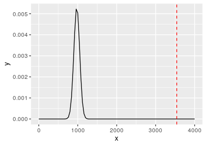
With the pval, we can see if it pass or fail the alpha threshold. Here because it is the first split, so alpha_level is 0.05. the fit$estimate[1] (mean) is 975 and fit$estimate[2] (sd) is 74.9.

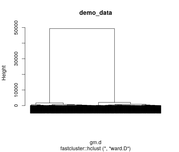
This time we can see that the Qclust (3541.71) is so far from the distribution of Qclust2 that the p-value is 0. And we can see that it makes sense to the hclust tree of the demo, that the first split led to 2 groups with extremely long branch!

Probability distribution of Qclust2. red line, Qclust value of the empirical data at first split

Conclusion

So this time I learnt about the concept of evaluating the validity of clustering based on the SCH concept. I learnt about generating on-demand PC using the scry package. Some of the ideas in crossprod and tcrossprod, especially in fit.model function is still confusing to me, but it is cool to see the codes for some ideas.

Finally, I learnt a lot about how to generate a log normal poison distribution, the code really helps. And next time, I will definitely try to use SCH-sc to rate the confidence of the clustering of my scRNA-seq data.