Using DMD model to identify response signature gene

Hasnain et al (2023) was interested in finding sensors for a pesticide called malathion that is usually present in micro-molar concentration ( 1.29 uM) in the environment. They performed time-series RNA-seq on the soil bacteria strain SBW25 for 80 minutes with up to 9 time points.

The interesting part is that they formulated an alternative way to analyse this time-series RNA-seq datasets that put the genes into groups (modes), captured their trajectories accurately and rank the genes within a mode based on their weights in the model.

In the results, they successfully identified 10 modes upon malathion induction and 15 biomarker genes that can serve as sensors for malathion.

Dynamic mode decomposition (DMD)

Proctor and Eckhoff had written a comprehensive review on the DMD method. In generate, it is a linear system that relate 2 time-state by

K_x = AK_{x + 1}

Well, actually, A looks like a transition matrix to me for MCMC processes. And finding the solution of A as components of eigenvectors of eigenvalues is somewhat like performing a PCA that decompose the high-dimensional data to dynamic modes. The eigenvalues and vectors describes the behavior of the mode and the element in the eigenvector describe its contribution towards the particular transformation.

Hasnain et al (2023) pointed out that the merit of DMD is that its sensitivity and effectiveness on selecting transcriptional responsible genes are high. One interesting finding is that when the malathion datasets were analysed using DeSeq2, only 5 significant DE genes were found. In contrast, their DMD methods identified 180 “DE” genes based on model weights. DMD model also selected a different DE gene list that only show an overlap of 31 genes with DeSeq2 results. They reasoned that DeSeq2 methods required more biological replicates and thus were insensitive when dealt with their 2-replicates datasets.

So DMD seems to be an attractive method to identify DE genes along with DeSeq2. Luckily the authors have shared their code and generated a tutorial in the github. So lets have a look.

DMD tutorial

import numpy as np
import pandas as pd
import seaborn as sns
import scipy as sp
from copy import deepcopy    
import matplotlib.pyplot as plt
import matplotlib
plt.rcParams.update({'font.size':25});
plt.rcParams.update({'axes.linewidth':1.5})
plt.rc('lines',linewidth=3);
from preprocess import *
from dmd import *
from sensor_placement import *
### load data 
df = pd.read_csv('data/GSE8799_series_matrix.txt',sep='\t')
ids = list(df['ID_REF'])
wt_df = df.iloc[:,1:df.shape[1]//2+1]
mt_df = df.iloc[:,list(np.arange(31,df.shape[1]))]
wt_df = np.log2(wt_df)
mt_df = np.log2(mt_df)
wt_df = np.array(wt_df).reshape(len(wt_df),15,2) # 15 timepoints, 2 replicates
mt_df = np.array(mt_df).reshape(len(wt_df),15,2) # 15 timepoints, 2 replicates

The tutorial has 2 part, the first half is individual analysis on mutant and WT state, and the later is the integrated analysis of WT vs Mutant. Sp lets have a look.

### WT
r = 10 # number of dynamic modes
A_wt,A_wt_red,wt_red,U_wt,_,eVals_r_wt,eVecs_r_wt,Phi_wt,b_r0_wt,b_r1_wt = \
        dmd(wt_df,rank_reduce=True,r=r,trim=False,trimThresh=2.5e-3)

### mutant 
r = 10 # number of dynamic modes
A_mt,A_mt_red,mt_red,U_mt,_,eVals_r_mt,eVecs_r_mt,Phi_mt,b_r0_mt,b_r1_mt = \
        dmd(mt_df,rank_reduce=True,r=r,trim=False,trimThresh=2.5e-3)

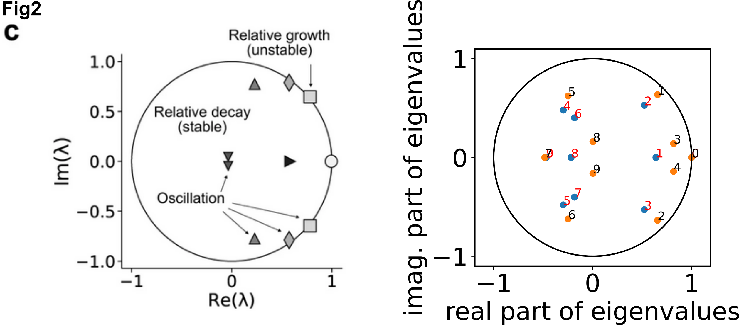
Calling the dmd function generated the eigenvalues(eVals:(10, )), eigenvectors(eVecs:(10, 10)) and the amplitude b from the time series data. Plotting the eigenvalues we can decide whether the eigenvalues are useful as a stable dynamic mode that fall within the circle.

Eigenvalues location in the unit circle.

nT = 15 
G_wt, G_recon_wt = gram_matrix(A_wt_red,wt_red[:,0,:],nT=nT,reduced=True,projection_matrix=U_wt)
G_mt, G_recon_mt = gram_matrix(A_mt_red,mt_red[:,0,:],nT=nT,reduced=True,projection_matrix=U_mt)
D_wt, V_wt = sp.linalg.eig(G_wt,left=False,right=True)
D_mt, V_mt = sp.linalg.eig(G_mt,left=False,right=True)
### ranking genes ###
w_wt = (U_wt @ V_wt)
w_mt = (U_mt @ V_mt)

So in w_wt((10928, 10)) and w_mt((10928, 10)) we get the weight of the genes in each of the mode.

rank_wt = np.argsort(w_wt[:, 0])
>>>rank_wt[::-1]
array([ 6273, 10035,  6209, ...,  7172, 10641,  8757])
>>>ids[rank_wt[::-1]]
array(['1775715_s_at', '1779562_at', '1775650_s_at', ..., '1776636_s_at',
       '1780178_s_at', '1778260_at'], dtype=object)
rank_wt = np.argsort(w_wt[:, 1])
>>>rank_wt[::-1]
array([8424, 8979, 9407, ..., 5352, 5586, 8642])
rank_wt = np.argsort(w_wt[:, 2])
>>>rank_wt[::-1]
array([  672,   144,  1408, ..., 10716, 10717, 10795])
### plot
fig, ax = plt.subplots(1,3,figsize=(14,5),sharex=True,sharey=False)
ax[0].set_title('Mode 0 WT')
ax[0].plot(np.mean(wt_df[6273],axis=1))
ax[0].plot(np.mean(wt_df[10035],axis=1))
ax[1].set_title('Mode 1 WT')
ax[1].plot(np.mean(wt_df[8424],axis=1))
ax[1].plot(np.mean(wt_df[8979],axis=1))
ax[2].set_title('Mode 2 WT')
ax[2].plot(np.mean(wt_df[672],axis=1))
ax[2].plot(np.mean(wt_df[144],axis=1))
plt.tight_layout()
plt.show()

fig, ax = plt.subplots(1,3,figsize=(14,5),sharex=True,sharey=False)
ax[0].set_title('Mode 0 WT')
ax[0].plot(np.mean(wt_df[8757],axis=1))
ax[0].plot(np.mean(wt_df[10641],axis=1))
ax[1].set_title('Mode 1 WT')
ax[1].plot(np.mean(wt_df[5586],axis=1))
ax[1].plot(np.mean(wt_df[8642],axis=1))
ax[2].set_title('Mode 2 WT')
ax[2].plot(np.mean(wt_df[10717],axis=1))
ax[2].plot(np.mean(wt_df[10795],axis=1))
plt.tight_layout()
plt.show()

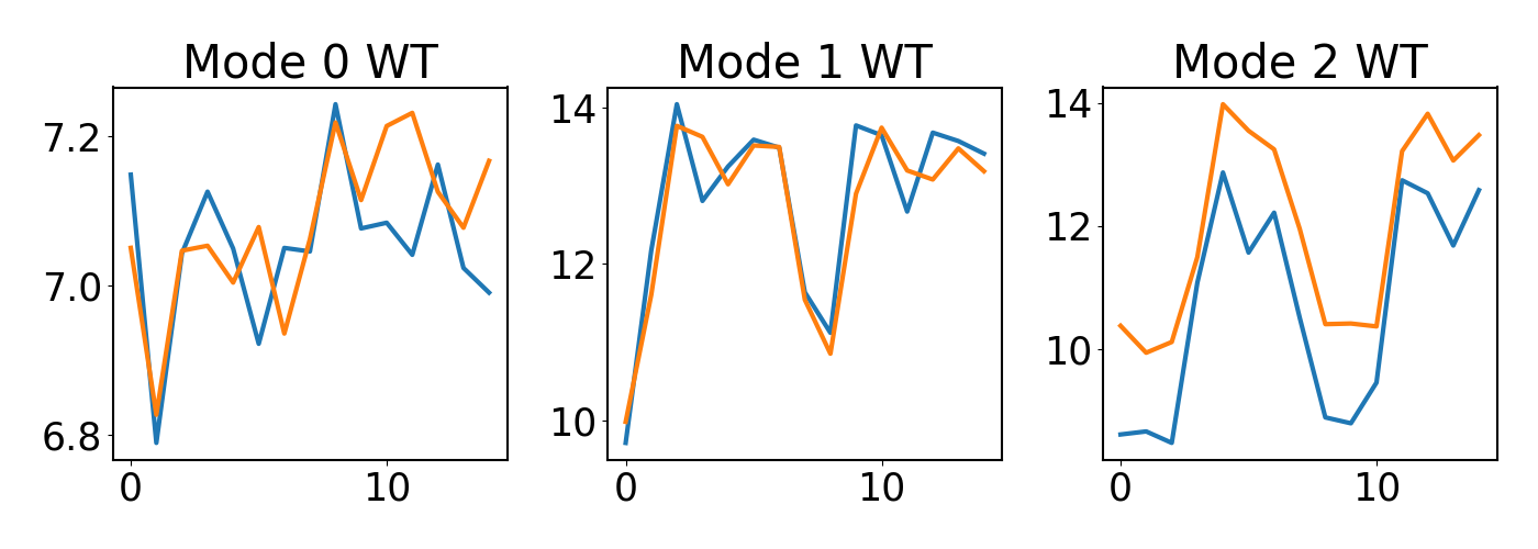
So it is quite cool to see that different Mode nominated Genes with distinct patterns and the top genes do show similar expression patterns for each mode.
But contrary to the paper’s claim that genes with lower weights show steady expression over time.the bottom genes of mode 1 and 2 do show distinct patterns…

So lets move on to the 2nd part of the tutorial that work on DE data.

wt_df = df.iloc[:,1:df.shape[1]//2+1]
mt_df = df.iloc[:,list(np.arange(31,df.shape[1]))]
wt_df = np.array(wt_df).reshape(len(wt_df),15,2) # 15 timepoints, 2 replicates
mt_df = np.array(mt_df).reshape(len(wt_df),15,2) # 15 timepoints, 2 replicates
fc = mt_df / wt_df
fc_orig = deepcopy(fc)
r = 20 # number of dynamic modes
A,A_red,fc_red,U,_,eVals_r,eVecs_r,Phi,_,_ = \
        dmd(fc,rank_reduce=True,r=r,trim=False,trimThresh=2.5e-3)

nT = 15 
G, _ = gram_matrix(A_red,fc_red[:,0,:],nT=nT,reduced=True,projection_matrix=U)
D, V = sp.linalg.eig(G,left=False,right=True)
w = (U @ V)
rank_w = np.argsort(w[:, 0])
>>>rank_w[::-1]
array([  863,  3250,  1633, ...,  3786, 10795, 10797])
rank_w = np.argsort(w[:, 1])
>>>rank_w[::-1]
array([10797, 10795, 10716, ...,  5118,   490,   657])
rank_w = np.argsort(w[:, 2])
>>>rank_w[::-1]
array([  657,  3786,  7064, ..., 10766, 10439,  2600])
rank_w = np.argsort(w[:, 5])
>>>rank_w[::-1]
array([10766,  1202,  5403, ..., 10222,   490,  7064])

fig, ax = plt.subplots(2,2,figsize=(14,5),sharex=True,sharey=False)
ax[0,0].set_title('Mode 0 DE')
ax[0,0].plot(np.mean(fc_orig[863],axis=1))
ax[0,0].plot(np.mean(fc_orig[3250],axis=1))
ax[0,1].set_title('Mode 1 DE')
ax[0,1].plot(np.mean(fc_orig[10797],axis=1))
ax[0,1].plot(np.mean(fc_orig[10795],axis=1))
ax[1,0].set_title('Mode 2 DE')
ax[1,0].plot(np.mean(fc_orig[657],axis=1))
ax[1,0].plot(np.mean(fc_orig[3786],axis=1))
ax[1,1].set_title('Mode 5 DE')
ax[1,1].plot(np.mean(fc_orig[10766],axis=1))
ax[1,1].plot(np.mean(fc_orig[1202],axis=1))
plt.tight_layout()
plt.show()

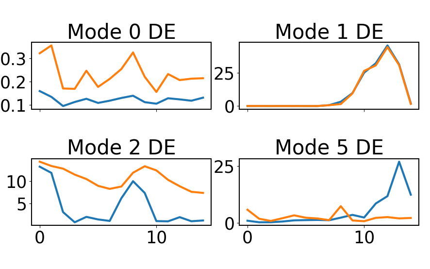
This time it looks like Mode 1 top genes have a more consistent patterns than the other modes examined.

Conclusion

Going through the DMD tutorials and reading the DMD papers, I am convinced that it is an effective methods to group genes based on expression patterns. And it seems to be an effective way to rank genes within a mode.

I would like to see how this method can be extended into GRN construction or at least somehow link functionally related genes together.