SCEPTRE improves calibration and sensitivity in single-cell CRISPR screen analysis
·Tackling high MOI single-cell crispr screen
State-of-art single cells perturb-seq and ECCITE-seq are very useful tools for dissecting gene function in a high throughput manner.
However, sorting out which gene-knockout effect as the real attribute to a gene expression change is very complicated.
Here, the authors of SCEPTRE (github, paper) looked into two high-MOI CRISPRi screens on enhancers and found that technical noise and expression disparity generate false positives. More specifically, they paired non-targeting sgRNA to a gene or sgRNA that are further than 1Mb away from the target protein coding gene and tested if the expression change is significant under such non-relationship. Some of these sgRNA-gene pair exhibit high level of dispersion and the sgRNA pairing region was mistaken as significant cis-regulator.
The authors found that the problem was stemmed from the way of handling the mean-dispersion relationship of gene expressions and proposed the package SCEPTRE to directly test the sgRNA-effect on gene expression in a pairwise manner. They also streamline the math framework to speed up the computation.
Concept of SCEPTRE
The typical way of gene-expression correction from raw count/UMI of a gene per cell is to fit a negative binomial distribution on the gene expression values of a gene to model the mean and dispersion of the gene.
Here lets follow what the paper did and first look into the DE calculation of monocle. Monocle instead fill a generalised linear model on gene expression over time.
$\ log(y_i) = \beta_i + \beta_t * x_t$
,where $\beta_t$ is the effect variable.
library(sceptre)
exps<-data("expressions")
sgRNA<-data("gRNA_indicators")
meta_data<-data("covariate_matrix")


library(sceptre)
data("expressions")
data("gRNA_indicators")
data("covariate_matrix")

exps<-matrix(expressions, nrow=1)
rownames(exps)<-"sceptre_exp"
colnames(exps)<-paste0("cell_", rownames(covariate_matrix))
rownames(covariate_matrix)<-paste0("cell_", rownames(covariate_matrix))
library(tidyverse)
covariate_matrix<-bind_cols(covariate_matrix, gRNA_indicators)
colnames(covariate_matrix)[6]<-"sgRNA"
genes<-data_frame(gene_short_name="sceptre_exp")
rownames(genes)<-"sceptre_exp"
library(monocle)
library(Matrix)
cds <- newCellDataSet(Matrix(exps, sparse=T),
                      phenoData =  new("AnnotatedDataFrame", data =covariate_matrix),
                      featureData = new("AnnotatedDataFrame", data =genes))

cds <- estimateSizeFactors(cds)
diff_test_res <- differentialGeneTest(cds, fullModelFormulaStr = "~sgRNA", relative_expr = F)

#status           family         pval         qval gene_short_name
#sceptre_exp     OK negbinomial.size 1.803409e-08 1.803409e-08     sceptre_exp
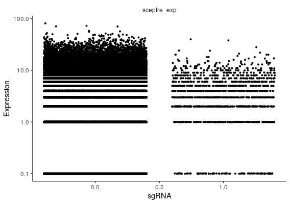
plot_genes_jitter(cds, grouping = "sgRNA", ncol=1, relative_expr = F)

Using the raw values from the expression matrix, monocle has found the example gene from SCEPTRE is highly DE with p-value of 1.8 x e-8.
SCEPTRE takes a different approach that fit the NB distribution with the rest of the covariate matrix, while these batch effects and technical noises are supposed to be corrected in the preprocessing step in monocle, i think.
result <- run_sceptre_gRNA_gene_pair(expressions = expressions,
                                      gRNA_indicators = gRNA_indicators,
                                      covariate_matrix = covariate_matrix,
                                      B = 1000,
                                      seed = 1234,
                                      reduced_output = FALSE)

result$p_value
#> [1] 0.2138241
So here, this gene does not show DE upon CRISPRi of the sgRNA according to SCEPTRE.p_value
NB test
To look into the matter, lets try to perform a typical NB fit for the data
require(foreign)
require(ggplot2)
require(MASS)
test_tab<-bind_cols(as.data.frame(covariate_matrix), t(exps))
colnames(test_tab)[7]<-"exps"
m1<-glm.nb(exps ~ sgRNA+p_mito+prep_batch+lg_total_umis+lg_guide_count+lg_n_genes, data=test_tab)
summary(m1)

Call:
glm.nb(formula = exps ~ sgRNA + p_mito + prep_batch + lg_total_umis +
    lg_guide_count + lg_n_genes, data = test_tab, init.theta = 3.1214302,
    link = log)

Deviance Residuals:
    Min       1Q   Median       3Q      Max
-3.0731  -0.8772  -0.2278   0.4253   6.7350

Coefficients:
                        Estimate Std. Error  z value Pr(>|z|)
(Intercept)            -7.860150   0.059160 -132.863   <2e-16 ***
sgRNA                  -0.006248   0.020481   -0.305     0.76
p_mito                 -4.068362   0.107928  -37.695   <2e-16 ***
prep_batchprep_batch_2  0.223456   0.003440   64.957   <2e-16 ***
lg_total_umis           0.587953   0.010977   53.563   <2e-16 ***
lg_guide_count          0.083920   0.003068   27.351   <2e-16 ***
lg_n_genes              0.404372   0.017862   22.638   <2e-16 ***
---
Signif. codes:  0 ‘***’ 0.001 ‘**’ 0.01 ‘*’ 0.05 ‘.’ 0.1 ‘ ’ 1

(Dispersion parameter for Negative Binomial(3.1214) family taken to be 1)

    Null deviance: 284298  on 205796  degrees of freedom
Residual deviance: 225926  on 205790  degrees of freedom
AIC: 966417

Number of Fisher Scoring iterations: 1


              Theta:  3.1214
          Std. Err.:  0.0181

 2 x log-likelihood:  -966400.5310


m2 <- update(m1, . ~ . - sgRNA)
anova(m1, m2)
Likelihood ratio tests of Negative Binomial Models

Response: exps
                                                                      Model    theta Resid. df
1         p_mito + prep_batch + lg_total_umis + lg_guide_count + lg_n_genes 3.121429    205791
2 sgRNA + p_mito + prep_batch + lg_total_umis + lg_guide_count + lg_n_genes 3.121430    205790
     2 x log-lik.   Test    df   LR stat.   Pr(Chi)
1       -966400.6
2       -966400.5 1 vs 2     1 0.09325092 0.7600843
The glm nb showed us that sgRNA has no effect at all; instead mitochondria gene % (aka cell quality) has a more profound effect.
REsampling from the NB Z-score
The key idea of SCEPTRE is the per-mutation test of sgRNA-expression pair. Here let try to illustrate this process using normal glm.
r<-summary(m1)
r$coefficients[2, 3]
> [1] -0.305063
### Collect z value of sgRNAs
### iterate 25 times
Z_values=c()
nb_summary<-list()
for (i in 1:25){
  new_test<-data_frame(sgRNA=sample(test_tab$sgRNA), exps=test_tab$exps)
  m1<-glm.nb(exps ~ sgRNA, data=new_test)
  r<-summary(m1)
  Z_values<-c(Z_values, r$coefficients[2, 3])
  nb_summary[[i]]<-r  }

### fit Z-scores to a normal distribution
> mean(Z_values)
[1] 0.3229951
> sd(Z_values)
[1] 0.792917
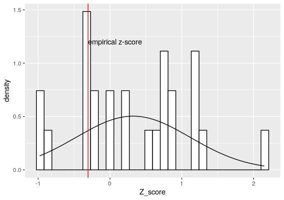
dnorm(-0.305, mean = mean(Z_values), sd = sd(Z_values))
[1] 0.3676814
### not significant

Simplified NB model by SCEPTRE
So using the SCEPTRE idea, by resampling the Z-score of the sgRNA effect, we can see that this sgRNA-gene pair is not significant. This is the beauty of SCEPTRE, rather than fixating on the Z_score assumption that it is somewhere around 0, SCEPTRE actually build a Z-score distribution using the empirical data while randomizing the sgRNA value.
This is actually very useful as now all the other technical noise is taken care of and we can directly evaluate the gene effect.
The even cleverer part is that SCEPTRE speed up the assessment by simplifying the calculation of comparing the NB regression with and without the sgRNA effect: NB(Yi ~ &Beta0 + technical effects) + NB(Yi ~ &Beta0 + sgRNA+ technical effects) = C + NB(Yi ~ &Beta0 + technical effects),
where C encompasses the sgRNA effect.
In this light, we can just fit the NB on data with sgRNA ==1 + technical effect and collect the Z_scores of the intercept. Because the resampling will reassign the sgRNA attribute, we will fruther reduce the input sample size.
Put simply, we first fit a NB on the read data of cell sgRNA==1, get the Z-score of the intercept. Then, we resample the data by randoming assigning some cells as sgRNA==1 (so each resampling has the same sample size as the real data) and fit the NB model to collect a set of Z-scores.
We can see this in the SCEPTRE raw code:
### in run_gene_precomputation
## first fit expression to NB distribution
fit_nb <- MASS::glm.nb(formula = expressions ~ ., data = covariate_matrix[, c("p_mito", "prep_batch", "lg_total_umis", "lg_guide_count", "lg_n_genes")])
fitted_vals <- as.numeric(fit_nb$fitted.values)
gene_precomp_size <- fit_nb$theta
gene_precomp_offsets <- log(fitted_vals)
### run_sceptre_using_precomp
# compute the test statistic on the real data
  fit_star <- VGAM::vglm(formula = expressions[gRNA_indicators == 1] ~ 1, family = VGAM::negbinomial.size(gene_precomp_size), offset = gene_precomp_offsets[gRNA_indicators == 1])
  t_star <- VGAM::summaryvglm(fit_star)@coef3["(Intercept)", "z value"]

  # Define a closure to resample B times (omitting the NAs)
  resample_B_times <- function(my_B) {
    t_nulls <- sapply(1:my_B, function(i) {
    ### resample sgRNA_indicator based on probability of 1, 0 exsistence ###
      gRNA_indicators_null <- stats::rbinom(n = length(gRNA_precomp), size = 1, prob = gRNA_precomp)
    ### fit NB using the randomized gRNA indicator as null_model ###
     fit_null <- VGAM::vglm(formula = expressions[gRNA_indicators_null == 1] ~ 1, family = VGAM::negbinomial.size(gene_precomp_size), offset = gene_precomp_offsets[gRNA_indicators_null == 1])
        VGAM::summaryvglm(fit_null)@coef3["(Intercept)", "z value"]},
        error = function(e) return(NA),
        warning = function(w) return(NA)
      )
    })
    t_nulls[!is.na(t_nulls)] ### collect all zscores from the null models
  }
A null_distribution of the z-score is built and the empirical Z-score (t_star in the code) is compared to the null_distribution to get the probabiliy of whether the chance of obtaining this Z-score is < 0.05.
Conclusion
I think SCEPTRE is a piece of very elegant work. A few small changes in the model has profound effect in helping clean up the data so well.
Also, understanding the code helped me to have a better understading in NB regression too, win.