The ultimate genotype-phenotype mapping made possible by synthetic library and Machine learning.

I came across this paper by Vaishnav et al and is so amazed on how ML is applied in evolutionary biology these days. It does not only predict, but also explain how adaptation and other driving forces are shaping the sequence. It is so cool, so let’s dive into it.

Objective

Description of the complete empirical fitness landscape of promoter sequences in yeste. foster new promoter design.
Using ML models to learn from a massive-parallel profile of yeast promoter regions (-160 to -80bp).

Advances.

One of the ML assisted genotype-phenotype mapping papers that have extensive discussion on evolution.
Very interesting way to perform summary statistics to answer evolutionary questions, tackling the mutation dynamics on expression changes.
Great use of the yeast genome resources!
New representation of evolvability!

A ‘gigantic’ parallel reporter assay of random DNA - previous paper

The data is from an extremely comprehensive paper (de Boer et al. 2019) on TF binding motifs the authors published previously.

Using “80bp of random DNA is expected to have, on average, ~138 partly overlapping TFBS instances, representing ~68 distinct factors.”, the authors charted the expression levels of each of the 10⁸ variants, arbeit still covering a small portion of the 4⁸⁰ variant space. This yielded high-resolution expression measurement for over 20 million randomly sample 80bp promoter sequences via FACS on YFP fluoresence reporter into 18 bins. Deep sequencing of each bin was then performed and the authors only worked with promoter sequences with at least 100 reads. The random N⁸⁰ sequences were then consolidated into a single consensus via self aligning via Bowtie2. “To collapse related promoters into a single representative sequence, we aligned the sequences observed in each library to themselves using Bowtie2 (version 2.2.1)56, creating a Bowtie database containing all unique sequences observed in the experiment (default parameters),” Any sequences that aligned to each other were assigned to the same cluster using CD-hit! It was not very obviously written in the main text, but I guess how that is done is to isolate the N⁸⁰ from the sequence using conserved flanking regions; use CD-hit to cluster sequences to make consensus. Then use the consensus to generate a bowtie2 reference for the final alignment. At the end, we will have the read-count for each consensus sequences per bin to calculate expression level.

“Expression levels for each promoter sequence were estimated as the weighted average of bins in which the promoter was observed. For those observed only once, the expression level was the center of the observed bin.”

wait what? weighted average - weight = proportion? so bin (avg expression) x read count?

So, this paper on its own has some valuable tactics on handling deep sequencing data and it definitely is worth coming back to study the methods more thoroughly.

This paper: deep transformer neural network capturing features of promoter sequences.

Now using this gigantic paper, they turn to use this data to look into some evolutionary theories on promoter sequences. First, they decided to reconstruct the full fitness landscape from empirical data on N⁸⁰ and natural yeast (multi-strains) promoters sequences.

According to the paper, the model contains 3 blocks: 1) generate useful features for forward and reverse strands of the random sequences; 2) capture interaction between strands (TFBM among both strands?) and 3) TF-TF cooperativity. Thankfully, the codes are posted in github as ipynb notebook and we can have a look at how they actually do this, with Supplementary Figure S1 as a guide of the model architecture.

def seq2feature_fill(i):
	""" ONE hot encoding of DNA"""
    mapper = {'A':0,'C':1,'G':2,'T':3,'N':None}
    ###Make sure the length is 110bp
    if (len(OHCSeq.data[i]) > 110) :
        OHCSeq.data[i] = OHCSeq.data[i][-110:]
    elif (len(OHCSeq.data[i]) < 110) : 
        while (len(OHCSeq.data[i]) < 110) :
            OHCSeq.data[i] = 'N'+OHCSeq.data[i]
    for j in range(len(OHCSeq.data[i])):
        OHCSeq.transformed[i][0][j][mapper[OHCSeq.data[i][j]]]=True 
    return i

### Padding of the consensus sequences extracted by CD-hit ###
sequences = [di[0] for di in d]
### Append N's if the sequencing output has a length different from 17+80+13 (80bp with constant flanks)
for i in tqdm(range(0,len(sequences))) : 
    if (len(sequences[i]) > 110) :
        sequences[i] = sequences[i][-110:]
    if (len(sequences[i]) < 110) : 
        while (len(sequences[i]) < 110) :
            sequences[i] = 'N'+sequences[i]


onehot_sequences = seq2feature(np.asarray(sequences))

tab = str.maketrans("ACTGN", "TGACN")

### Also make on-hot encoding for reverse complement###
def reverse_complement_table(seq):
    return seq.translate(tab)[::-1]

rc_sequences = [reverse_complement_table(seq) for seq in tqdm(sequences)]

rc_onehot_sequences = seq2feature(np.array(rc_sequences))

These preprocessing steps generate the sequence input for the first block of the ML. The final one-hot encoding has a dimension of 4: (shared_array.reshape(len(data),1,len(data[0]),4)): len(data)=entry of samples; 1: per sample; len(data[0])= 80+30bp padding of each sample, 4: A/T/G/C binary matrix.
It seems like that they did not normalise the expression data. So now let’s examine the model architecture.

def cnn_model(X, hyper_params , scope):

    with tf.variable_scope(scope) : 
        global _hidden 
        conv1_filter_dim1 = 30
        conv1_filter_dim2 = 4
        conv1_depth = _hidden
        conv2_filter_dim1 = 30
        conv2_filter_dim2 = 1
        conv2_depth = _hidden


        W_conv1 = weight_variable([1,conv1_filter_dim1,conv1_filter_dim2,conv1_depth])
        conv1 = conv2d(X, W_conv1)    
        conv1 = tf.nn.bias_add(conv1, bias_variable([conv1_depth]))
        conv1 = tf.nn.relu(conv1)
        l_conv = conv1
        
        W_conv2 = weight_variable([conv2_filter_dim1,conv2_filter_dim2,conv1_depth, conv2_depth])
        conv2 = conv2d(conv1,W_conv2 )
        conv2 = tf.nn.bias_add(conv2, bias_variable([conv2_depth]))
        conv2 = tf.nn.relu(conv2)

        
        regularization_term = hyper_params['l2']* tf.reduce_mean(tf.abs(W_conv1)) + hyper_params['l2']* tf.reduce_mean(tf.abs(W_conv2)) 
        
        cnn_model_output = conv2

    return cnn_model_output , regularization_term 

The first layer, it is quite interesting that the kernel that has 30 features, would be good if someone can explain why and how to choose kernel dimension…..

### in def training()
#f is forward sequence 
    output_f , regularization_term_f =  cnn_model(X, {'dropout_keep':hyper_params['dropout_keep'],'l2':hyper_params['l2']} , "f")

    #rc is reverse complement of that sequence
    output_rc , regularization_term_rc =  cnn_model(X_rc, {'dropout_keep':hyper_params['dropout_keep'],'l2':hyper_params['l2']} , "rc")
    
    
    ### CONCATENATE output_f and output_rc
    concatenated_f_rc = tf.concat([output_f , output_rc], -1)
    ###

So here, it look like they put the CNN features of reverse and forward strand together. Then feed the features into layer 2.

W_conv3 = weight_variable([conv3_filter_dim1,conv3_filter_dim2,2*_hidden,conv3_depth])
    conv3 = conv2d(concatenated_f_rc,W_conv3 )
    conv3 = tf.nn.bias_add(conv3, bias_variable([conv3_depth]))
    conv3 = tf.nn.relu(conv3)

    W_conv4 = weight_variable([conv4_filter_dim1,conv4_filter_dim2,conv3_depth,conv4_depth])
    conv4 = conv2d(conv3,W_conv4 )
    conv4 = tf.nn.bias_add(conv4, bias_variable([conv4_depth]))
    conv4 = tf.nn.relu(conv4)


    conv_feat_map_x = 110   
    conv_feat_map_y =  1   
    h_conv_flat = tf.reshape(conv4, [-1, conv_feat_map_x * conv_feat_map_y * lstm_num_hidden])

There are 2 more layers of CNN with 64 Hidden Units, each consisting of ReLU and Dropout (0.05 dropout probability), then the representation is reshaped bakc to (110, 1) = sequence length?.

#Transformer Encoder Blocks.
    
    W_fc1 = weight_variable([conv_feat_map_x * conv_feat_map_y * lstm_num_hidden , fc_num_hidden])
    b_fc1 = bias_variable([fc_num_hidden])
    h_fc1 = tf.nn.relu(tf.matmul(h_conv_flat, W_fc1) + b_fc1)
    #Dropout for FC-1
    h_fc1 = tf.nn.dropout(h_fc1, dropout_keep_probability)

    
    #FC-2
    W_fc2 = weight_variable([fc_num_hidden , num_bins])
    b_fc2 = bias_variable([num_bins])
    h_fc2 = tf.nn.relu(tf.matmul(h_fc1, W_fc2) + b_fc2)
    #Dropout for FC-2
    h_fc2 = tf.nn.dropout(h_fc2, dropout_keep_probability)

    #FC-3
    W_fc3 = weight_variable([num_bins, num_classes])
    b_fc3 = bias_variable([num_classes])
    h_fc3 = tf.matmul(h_fc2, W_fc3) + b_fc3 

I am a bit confused there, the paper said there are 2 transformer block, but it looks like there are 3? Anyway, the output is “Linear Combination of the 256 features extracted as a result of all the previous operations on the sequence (s) to generate the predicted expression (e).”.

So are we from now on working with the 256 features and e? From the ga.ipynb it looks like I can input sequences and predict their expression. That quite departs from my expectation that the transformer Encoder can compute sequence as output… well nvm. In brief, using the ga algorithm, the full fitness landscape is now reconstructed and some interesting analyses can be done with it.

Computing Expression Conservation Coefficient (ECC) detects

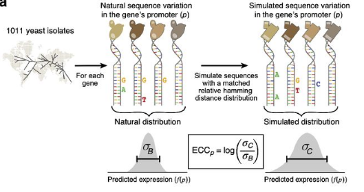
Now we arrive at the fun part. The authors derive the ECC score to compare mutations of natural sequences and N⁸⁰ sequences. The idea is to see if the expression variation (sd) is bigger or smaller among natural sequences compared to randomized synthetic sequences, as explained in figure 3A. Based on the natural sequences, a pool of selected variants of the consensus promoter are derived so that the number of sequences at each Hamming distance from the consensus promoter sequence was the same for the natural and simulated sets. Then a second set of random sequences that are restricted to 1 mismatch away from all natural occurring orthologues are sampled to make the correction fator C. And the corrected ECC is defined as log($/sigma$c/$/sigma$B) - C.

Histogram of f<sub>c</sub> — Fig. 3A of Vaishnav1 et al. The ECC for a gene is defined as log($\sigma$c/$\sigma$B) - C(constant correction factor)

That is actually kind of a breakthrough, as it goes beyond quantifying variations (dN/dS) in the promoter sequences but actually measuring the phenotypic plasticity of the promoter region of a gene. Now, we are not constrained to work with what are biological available, we can instead distill the evolutionary machanism that lead to the biological sequences we can observed today. High ECC ($\sigma$B is smaller than $\sigma$c) probably means conservation whereas low ECC probably means diversification.

After calculating the ECC of each gene, the model is useful to study the evolutionary aspect of promoter complexity. The authors found that high ECC is enriched in highly conserved cellular process while low ECC is enriched in adaptation related process.

“Thus, the ECC quantified stabilizing selection on expression in yeast and may even predict stabilizing selection on orthologs’ expression in other species. Genes”

Mutational robustness and evolvability

Next the authors looks into the portion of single nucleotide mutational neighbors of a consensus promoter that do not alter expression. They found that fitness responsivity (computed from the expression-to-fitness curves in glucose media, that’s another paper) positively correlated with mutational robustness of promoters.

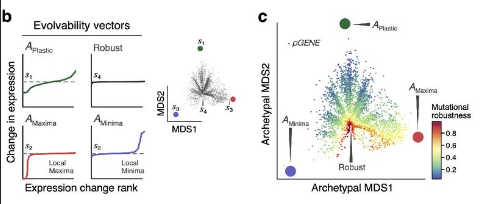
Finally, the authors looked into evolability. There, they ranked mutations according to the expression change of the single nucleotide mutation neighbors compared to the consensus. As explained in the maintext, evolvable promoters can easily change their expression with mutation (thus more extreme differences?) while robust promoter can tolerate many mutations with stable expressions. The authors use these vectors of expression differences derived for each consesnsus sequences to train an autoencoder. Using the autoencoder, they found that there are the robust type (minima, robust and maxima) and plastic promoter archetypes.

Then they feed the natural sequences into the autoencoder and found a strong negative correlation between a se- quence’s proximity to the plastic archetype and its mutational robustness.

Thoughts and conclusion

I think this paper really demonstrates how MAVE and ML can be used to address interesting questions in biology besides optimization problems.

This paper stands out in a way that its use of ML actually provide insights into the sequence’s evolutionary history and evolvability. It also provide us with a lot of useful details in analysing MAVE data, model building, summarizing orthologues sequences and interpreting ML models. It is so exciting to see that more and more evolution papers start to employ ML and perform more thought provoking analyses to test different evolutionary theories. There are still so much to unpack with this dataset and I do look forward to reading more discoveries on it.