Using Revolver to study cancer evolution.

The challenge in studying cancers

Cancer evolution, the accumulation of mutations driving the formation of carcinomas, is always fascinating and confusing at the same time. On one hand, it is fascinating to see that there are key oncogenes and tumor suppression mutations that show up repeatedly; while on another hand, each cancer has its own evolution trajectory that the driver genes mutations may not follow a general trend. Sampling biases and intra-tumor heterogeneity make conferring a correct phylogenetic tree even harder.

I began this post with reading about the Revolver package back in April. It is a tool to identify key evolutionary event in carcinogenesis via jointly analysing bulk multi-region samples. There, I not only learnt about a few new concepts on studying the heterogeneity and transition of cancers, I also learn about a few important packages to deconvolute the structural hierarchy of a tumor tissue sample via phylogenetic tree construction, CCF influence and B allele frequency estimations using NGS data. These are all very new to me, so I will go through them one by one.

Revolver take a bunch of trees inferred from multi-region tumor sequencing data of patients. It then identify recurrent mutations (important cancer drivers) and recurring evolution trajectory among patients; these repeated events must be key to cancer progression.

Revolver pipeline and input data

Revolver jointly handle data of multiple patients, each have multiple cancer regions sequenced sound exciting; this is a massive pipeline with a few cancer evolution concepts I need to learn about.

The first term is the cancer cell fraction (CCF). While CCF is vital in reconstructing the clonal relationships among cancer cells, CCF cannot be directly derived from variant allele frequencies due to copy number variations and subclone variations. In Revolver, it uses an adopted version of ClonEvol, which takes in a clustering cancer clones to infer phylogeny. Rather than taking the consensus clonal ordering, Revolver take the distribution of trees generated by ClonEvol plausible under the input clonal clustering as its input.

ClonEvol

ClonEvol aims at building a true clonal tree that support the subclone clustering from SNV and CNV information. The authors of ClonEvol pointed out that, the typical sum rule (the parental Clone CCF > sum of all subclone CCF) applied by classifying subclone can be easily violated due to sampling bias. The sum rule is an elaboration of the “pigeonhole principle”, which state that the number of pigeonholes has to be greater than that of the pigeons. In the application to subclonal architecture, when the sum of the subclone mutation frequencies exceed the parental clone frequency, the subclone with lower frequency must be descendant of the one with higher frequency. Such clonal relationship inference is summarized in ClonEvol Fig.1.

ClonEvol use bootstrap resampling to estimate parental clone CCF; and it assign a P_neg value to each potential parental clone. The more often the parental clone violates the sum rule in the bootstrap resampling, the bigger the P_neg. ClonEvol then use the P_neg values to evaluate trees reflecting all the possible clonal order and identify the most plausible tree with the least number of violating nodes.

The use of bootstrapping here is sound but I think one probably need to sequence a lot and have numerous high prevalence VAFs to perform ClonEvol. That kinda raise the fundamental question that how “good” the input clustering needs to be as input of ClonEvol; how we can attain such clustering and whether we are working with data having enough formative SNVs and CNVs to present a “reasonable” clustering.

PyClone

PyClone performs Bayesian clustering on bulk sequencing data of somatic mutations. The Dirichlet Process outperforms other clustering methods as we do not need to pre-define the number of cluster and it inform us the probablity of each member belonging to a particular cluster.

Briefly, pyclone organised mutations into clusters based on their VAF, using the dirichlet process. This clustering output then is the input of Clonevol for clonal tree construction.

Testing the pipeline

So I tried out Pyclone-VI available in (github). I used the curated tracerx data in the examples directory for and follow the instructions to get the clustering output.

Looking into the TRACERx data, it is the resultant SNPs information from a sequencing project of 100 patients of non-small-cell lung cancer Jamal-Hanjani et al (2017).

It is a huge dataset consist of 3 sequencing samples (R1, R2, R3) from 427 tumour and control samples sequenced to 426x depth. The authors also reported the CCF, copy number variations, and other essential information that is required for Pyclone (reference counts, alternative counts, CNV for normal and cancer cells, and CCF of the sample). Mutation is named with patientID:chromosome:location:SNP_base format (i.e. CRUK0001:7:47971…).

Pyclone identified 7 clusters from the >7230 SNPs input. Now we proceed to try Clonevolv for clonal tree construction. Here, we follow the Clonevolv tutorial protocol

First we inspect the VAFs of various clusters among the 3 samples of the TRACERX dataset.

library(clonevol)
library(tidyverse)
library(ggplot2)
### try pyclone output
T<-read.csv("tracerx_pyclone_result.csv", stringsAsFactors = F, sep="\t")
### try to trun it to clonevolv accept format
Tracerx<-T %>% dplyr::select(mutation_id, cluster_id, sample_id, cellular_prevalence)
Tracerx$mutation_id<-gsub("b'", "", Tracerx$mutation_id)
Tracerx$mutation_id<-gsub("'", "", Tracerx$mutation_id)
Tracerx$sample_id<-gsub("b'", "", Tracerx$sample_id)
Tracerx$sample_id<-gsub("'", "", Tracerx$sample_id)
Tracerx<-Tracerx %>% spread(sample_id, cellular_prevalence)
Tracerx<-Tracerx %>% arrange(cluster_id)
Tracerx<-Tracerx %>% mutate(R1=R1*100, R2=R2*100, R3=R3*100)
plot.variant.clusters(Tracerx, cluster.col.name = "cluster_id", 
                      vaf.col.names = c("R1", "R2", "R3"))
plot.cluster.flow(Tracerx, cluster.col.name = "cluster_id",
                  vaf.col.names = c("R1", "R2", "R3"),
                  sample.names =c("R1", "R2", "R3"))

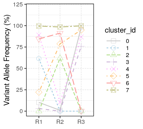
To infer clonal structure, I picked cluster 7 (the one with highest VAF) as the founder cluster and infer a “monoclonal” model. infer.clonal.model cannot accept 0-base cluster numbering, so each cluster number has 1 added. Then I run the “polyclonal” model without specifying the founder cluster.

y =infer.clonal.models(
  variants = Tracerx,
  cluster.col.name ='cluster',
  vaf.col.names =  c("R1", "R2", "R3"),
  founding.cluster=8,
  cancer.initiation.model='monoclonal',
  subclonal.test ='bootstrap',
  subclonal.test.model ='non-parametric',
  num.boots = 1000)

y =infer.clonal.models(
  variants = Tracerx,
  cluster.col.name ='cluster',
  ccf.col.names =  c("R1", "R2", "R3"),
  cancer.initiation.model='polyclonal',
  subclonal.test ='bootstrap',
  subclonal.test.model ='non-parametric',
  num.boots = 1000)

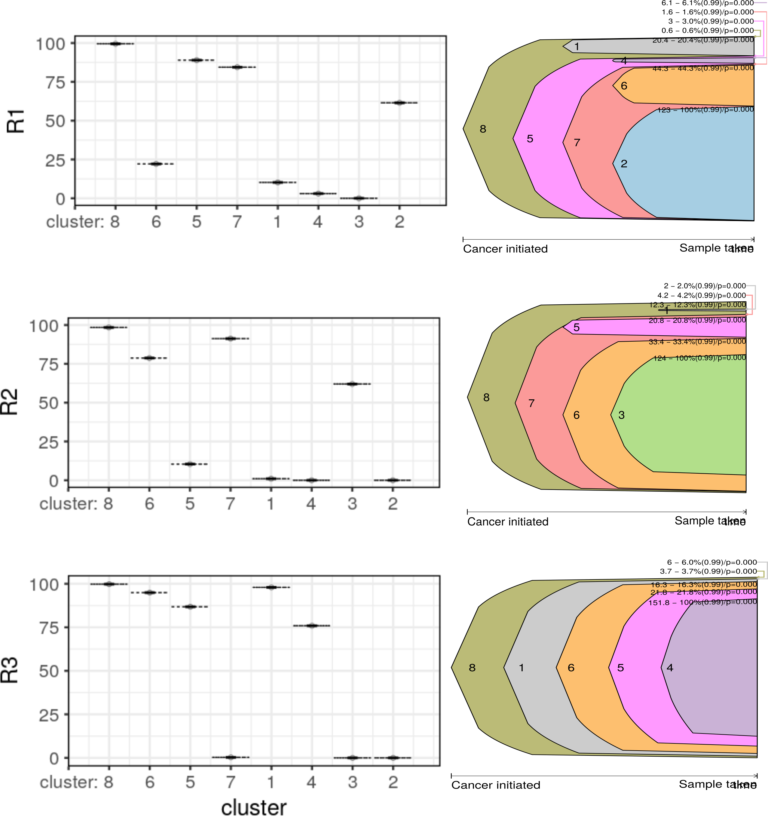
Clonevol found 37, 15, and 1 clonal model for R1, R2 and R3 using the “monoclonal” model and 44, 3, and 1 clonal models using the “polyclonal” model. No “consensus” models were found in neither settings, that’s not ideal. Interesting, I could only plot the fish plots of individual samples. Not sure what had gone wrong. I is quite interesting that R3 showed a perfect sequential order for cluster emergence. R1 and R2 have unstable inference of cluster 1, 4 and cluster 5, thus producing multiple inference. Both clusters are at the lower VAF end but not yet excluded from the model.

Try revolver

Now, let try revolver. The tutorial is at revolver/vignettes/Input_formats.Rmd, Getters.Rmd and Plotting_functions.Rmd. It is also using the TRACERX data as an example. Revolver has another specific format for the input. It require patient ID for a specific SNP, gene name, etc. The Pyclone cellular pervalence output is now specified in the CCF column for all samples.

install.packages("remotes")
remotes::install_github("caravagn/revolver")
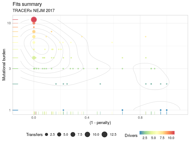
# Load an example dataset - the TRACERx cohort
data("TRACERx_NEJM_2017", package = "evoverse.datasets")
# This is a dataset that follows the specifications given above
print(TRACERx_NEJM_2017)

# A tibble: 65,421 x 7
   Misc              patientID variantID cluster is.driver is.clonal CCF   

   <chr>             <chr>     <chr>     <chr>   <lgl>     <lgl>     <chr>   
 1 CRUK0001:7:47971… CRUK0001  PKD1L1    1       FALSE     FALSE     R1:0.86;R2:…
 2 CRUK0001:21:4775… CRUK0001  PCNT      1       FALSE     FALSE     R1:0.86;R2:…
 3 CRUK0001:22:3733… CRUK0001  CSF2RB    1       FALSE     FALSE     R1:0.86;R2:…
 4 CRUK0001:10:1028… CRUK0001  KAZALD1   1       FALSE     FALSE     R1:0.86;R2:…
 # … with 65,411 more rows

require(tidyverse)
require(revolver)
subset_data = TRACERx_NEJM_2017 %>%
  filter(patientID %in% c("CRUK0001", "CRUK0002", "CRUK0003", "CRUK0004","CRUK000
                          5","CRUK0006", "CRUK0007","CRUK0008","CRUK0009","CRUK0010"))
# Create a cohort
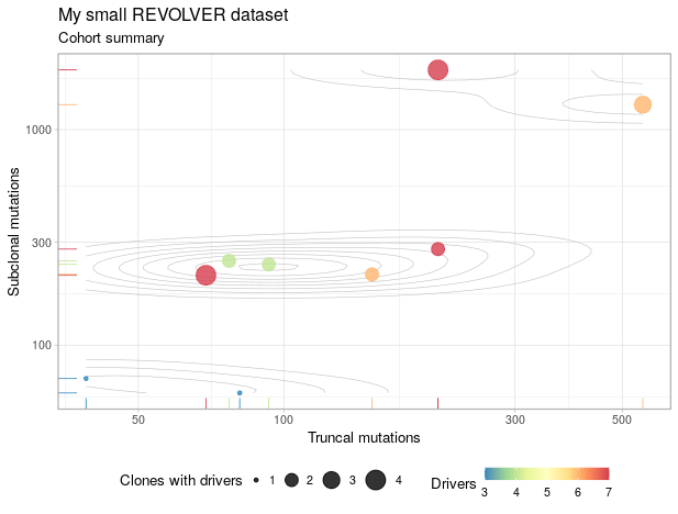
my_cohort = revolver_cohort(
  subset_data, 
  CCF_parser = CCF_parser,
  ONLY.DRIVER = FALSE, 
  MIN.CLUSTER.SIZE = 0,
  annotation = "My small REVOLVER dataset"
)
── Extracting clones table ──────────────────────────────────────────────────
→ CRUK0001 : 2100 entries, 11 clone(s).
→ CRUK0002 : 280 entries, 7 clone(s).
→ CRUK0003 : 330 entries, 7 clone(s).
→ CRUK0004 : 323 entries, 7 clone(s).
→ CRUK0006 : 1856 entries, 7 clone(s).
→ CRUK0007 : 109 entries, 3 clone(s).
→ CRUK0008 : 365 entries, 4 clone(s).
→ CRUK0009 : 487 entries, 10 clone(s).
→ CRUK0010 : 141 entries, 3 clone(s).

That’s very cool that revolver create a clonal structure of each patient. Here it outputs the clones info of patient 1 to 10 as I requested.

It also had the analysed TRACERx data of all 100 patients.

Revolver plot of the TRACERx cohort. Transfer: Information Transfer for the drivers. Drivers: Number of cancer driver each clone carries.

Conclusion

Here, I tried to look into how clonal structure of cancer clones are constructed using Pyclone, Clonevolv and revolver. It is definitely not easy to infer clonal relationship from SNPs data, hopefully single-cell sequencing later can help as SNPs clustering will be more confident using single-cell data.

I have a chance to work with a huge cancer cohort dataset; it is already a lot of effort to generate such precise and rich information. It is an invaluable resources and I am thankful that these dataset are maintained and documented so extensively, and made publicly available for software development and other future researches. That’s incredible!