Gemini - identify interacting genes from combinatorial CRISPR screens.
·Modeling gene-gene interactions from double knockouts.
MAGeCK is prevailing as the most popular software to test gene knockdown effects from CRISPR screen. As the cost of library construction drops, people are now building multiplexed constructs containing multiple sgRNAs that knock down at least two genes once introduced into a cell. We need software that can handle such multiplexed experiments, reporting effects of individual sgRNA as well as their joint effects.
Today, I am exploring GEMINI by Zamanighomi et al. (2019), which is the package specialised for double KO CRIRSPR screen. For comparison, we also look into the sgRNA interaction effects derived from the methods of Shen et al. (2017). Both methods focus on pairwise sgRNA designs and both have their codes publicly available. It will be very cool to learn about how they establish their models and if I could apply them later for multiplexed screen involving more than 2 sgRNAs.
Dual_crispr_pipeline from Shen et al. (2017)
I am still fresh in modeling, so just looking at the paper’s method session did not really help me to work out how the interaction is calculated. But the authors kindly uploaded their ipython notebooks so that I can learn more via digging through the code.
Briefly, the author calculate the fitness value fc at time t for each sgRNA-pair, that
xc=ac + fct
xc is the read composition of the sgRNA-pair, ac is the initial composition. So fc is a factor that cause acto increase or decrease over time.
After the fc values are derived, individual fitness effect of each gene and the gene-gene interaction score ($\pi$) are calculated:
fc = fgene1 + fgene2 + $\pi$gene1-gene2
In this step, the authors performed robust fitting to get the mean values of fgene and $\pi$.
The code
I could not find the relevant raw count table for Shen et al (2017), so I tried to fit the Big-Papi A549 data into the dual_crispr_pipeline notebook 6, where all the modeling are documented.
The code had a rigid format to accommodate the original dataset so it took me some time to clean up and apply it to the A549 data (plasmid + 2 replicate at end-point; 29 genes while and HPRT intron is targeted by 10 sgRNAs; total 192 sgRNA probes). I have also put all the code back to R so that I am only using Rstudio to execute the code. There are still several variables I am not sure if I have assigned correctly, as there were not enough explanation to work out what they are exactly. First of all, we prepare the data to fit into the dual_crispr_pipeline
library(MASS)
library(locfdr)
library(qvalue)
library(tidyverse)
library("gemini")
data("counts", "guide.annotation", "sample.replicate.annotation", package = "gemini")

### import counts
time<-c(0, 1) ### Big Papi have only 2 time points
X<-bind_cols(guide.annotation[, c("U6.gene", "H1.gene")], as.data.frame(counts[, c("pDNA", "A549.RepA", "A549.RepB")]))
colnames(X)[1:2]<-c("geneA", "geneB")
small<-1e-6 ### pseudocount
#preliminary preparations of the input data frame
data<-data.matrix(X[,3:5])
good<-(X$geneA != X$geneB) #reject any constructs with two 0's
goodX<-X[good,] #the 0-0 constructs are gone
nn<-sum(good) #this many constructs
### Sort out probes ###
goodX<-goodX %>% mutate(guides=rownames(goodX))
goodX<-goodX%>% separate(guides, c("sgRNA1", "sgRNA2"), sep=";")
### so in the Big Papi data, each sgRNA combination has 3 replicates, each gene is targeted by 3 sgRNA
probe_tab<-bind_rows(goodX %>% group_by(sgRNA1, geneA) %>% summarise(n()) %>% arrange(geneA) %>% mutate(sgRNA=sgRNA1, gene=geneA) %>% ungroup()%>%  dplyr::select(sgRNA, gene),
                     goodX %>% group_by(sgRNA2, geneB) %>% summarise(n()) %>% arrange(geneB) %>% mutate(sgRNA=sgRNA2, gene=geneB) %>% ungroup()%>% dplyr::select(sgRNA, gene))
probe_tab <-probe_tab[!duplicated(probe_tab), ]

goodX<-goodX %>% mutate(sgRNA1=paste(geneA, sgRNA1, sep="_"), sgRNA2=paste(geneB, sgRNA2, sep="_"))
### HPRT_intron and 6T shall be the nontargeting in this dataset
cpA<-as.character(goodX$sgRNA1)
ix<-grepl("6T", cpA) | grepl("HPRT intron", cpA)
cpA[ix]<-paste("0",cpA[ix],sep="") #this puts NonTargeting probes at the beginning of alphabetically sorted order
cpB<-as.character(goodX$sgRNA2)
ix<-grepl("6T", cpB) | grepl("HPRT intron", cpB)
cpB[ix]<-paste("0",cpB[ix],sep="")
### make sure cpA and cpB are in alphahbetical order
pswitch<-cpA>cpB #need to switch?
phold<-cpA[pswitch]
cpA[pswitch]<-cpB[pswitch]
cpB[pswitch]<-phold #cpA and cpB are always in alphabetical order, cpA < cpB
probes<-sort(unique(c(cpA,cpB))) #entire probe set in alphabetical order
nprobes<-length(probes)
### total 192 probes
cgA<-as.character(goodX$geneA)
cgB<-as.character(goodX$geneB)
genes<-sort(unique(cgA))
n<-length(genes)
mm<-n*(n-1)/2 ### 29 x 29 combinations
gA_gB<-paste(cgA,cgB,sep="_")
goodX<-data.frame(goodX,cgA,cgB,gA_gB) #now gA_gB is ordered so that gA < gB
gooddata<-data.matrix(goodX[,3:5])
gooddata[gooddata==0]<-1 #pseudocounts
abundance<-apply(gooddata,2,sum)
### compute estimates the relative abundance, Xc for each combination
y<-t(log2(t(gooddata)/abundance)) #log2 frequencies
This first step kept unique sgRNA-pairs, sort out the orders of interacting probes and genes, identify negative control genes, and calculate log2(relative abundance) of each sgRNA-pair.
### Abundance Threshold Selection
rge<-range(y)
for (i in 1:ncol(y)) {
  h<-hist(y[,i],breaks=seq(rge[1]-0.05,rge[2]+0.05,by=0.05),main=colnames(y)[i],xlab=expression(paste(log[2]," relative frequency")),col="grey80",border=FALSE)
  d<-density(y[,i],bw=0.2)
  lines(d$x,d$y*sum(h$counts)*0.05,col="black")
}
### set read theshold to -20 for all libraries ###
ab0<- c(-20, -20, -20)
### filter out sgRNA combinations with reads lower than threshold ###
g1names<-matrix("",ncol=n,nrow=n)
g2names<-matrix("",ncol=n,nrow=n)
ggnames<-matrix("",ncol=n,nrow=n)
for (i in 1:(n-1)) {
  for (j in (i+1):n) {
    g1names[i,j]<-genes[i]
    g2names[i,j]<-genes[j]
    ggnames[i,j]<-paste(genes[i],"_",genes[j],sep="")
    ggnames[j,i]<-ggnames[i,j]
  }
}

# for replicate 1
nt=2 ### 2 time points
x1<-y[,c("pDNA", "A549.RepA")]
ab1<-ab0[1:2]
bad1<-apply(t(x1)>ab1,2,sum)<2
print(sum(bad1))
# for replicate 2
x2<-y[,c("pDNA", "A549.RepB")]
ab2<-ab0[c(1, 3)]
bad2<-apply(t(x2)>ab2,2,sum)<2
print(sum(bad2))
Next, a low-abundance threshold for each sample are manually selected by looking at the abundance histogram. Those low-abundance sgRNA-pair are then removed from the analysis. Then, we generate table x1, and x2 for our two replicates.
Var<-function(x) mean(x^2)-mean(x)^2 #scalar version
vVar<-function(x) apply(x^2,1,mean)-apply(x,1,mean)^2 #vector version
Cov<-function(x,y) mean(x*y)-mean(x)*mean(y)
vCov<-function(x,y) apply(t(x)*y,2,mean)-apply(x,1,mean)*mean(y) #x is a matrix and y is a vector
sqrtsum<-function(y) sqrt(sum(y^2))
fit_ac_fc<-function(x1,ab1,x2,ab2) {
  #badx is TRUE when x-value is bad
  er_ac<-1
  l<-0
  nx<-nrow(x1)
  good1<-t(t(x1)>ab1)
  good2<-t(t(x2)>ab2)
  useless1<-apply(good1,1,sum)<2
  useless2<-apply(good2,1,sum)<2
  good1[useless1,]<-FALSE #remove singletons
  good2[useless2,]<-FALSE #remove singletons
  allbad<-apply(good1,1,sum)<2 & apply(good2,1,sum)<2 #in this case I have nothing to use in either experiment

  lambda1<-rep(0,nt)
  lambda2<-rep(0,nt)
  ac1<-x1[,1] #pDNA col
  ac2<-x2[,1] #pDNA col
  fc<-rep(0,nx)

  for (i in 1:nx) {
    ### calculate initial fc for each sgRNA combination for the pDNA ###
    if (allbad[i]) next #from now on there is at least one good experiment
    f1<-0
    f2<-0
    v1<-0
    v2<-0
    g1<-good1[i,]
    if (sum(g1)>1) { #it's a good experiment
      mx1<-mean(x1[i,g1]) ### mean between pDNA and treatment rep1
      mt1<-mean(time[g1])
      v1<-Var(time[g1])
      f1<-Cov(x1[i,g1],time[g1])
    }

    g2<-good2[i,]
    if (sum(g2)>1) { #it's a good experiment
      mx2<-mean(x2[i,g2])
      mt2<-mean(time[g2])
      v2<-Var(time[g2])
      f2<-Cov(x2[i,g2],time[g2])
    }
    fc[i]<-(f1+f2)/(v1+v2) #the combined fitness from replicate 1+2
    #fc remains defined up to an additive constant
    if (sum(g1)>1) {
      ac1[i]<-mx1-fc[i]*mt1
    }
    if (sum(g2)>1) {
      ac2[i]<-mx2-fc[i]*mt2
    }
  }

  alpha<- -log2(sum(2^ac1))
  ac1<-ac1+alpha #enforce normalization at time=0, sum(2^ac)=1
  alpha<- -log2(sum(2^ac2))
  ac2<-ac2+alpha #enforce normalization at time=0, sum(2^ac)=1

  for (i in 1:nt) {
    lambda1[i]<- -log2(sum(2^(ac1+fc*time[i])))
    lambda2[i]<- -log2(sum(2^(ac2+fc*time[i])))
  } #these are initial estimates of lambda(t)

### calculate expected LFC for each sgRNA combination ###
  xfit1<-x1 #for size
  for (j in 1:nt) {
    xfit1[,j]<-ac1+fc*time[j]+lambda1[j]
  }
  xfit2<-x2 #for size
  for (j in 1:nt) {
    xfit2[,j]<-ac2+fc*time[j]+lambda2[j]
  }
  sdfc<-rep(0.1,nx) #standard error of fc
  tstat<-rep(0,nx)
  df<-rep(0,nx)
  p_t<-rep(1,nx)
  for (i in 1:nx) {
    if (allbad[i]) next

    g1<-good1[i,]
    g2<-good2[i,]
    df[i]<-sum(g1)+sum(g2)-2
    sdfc[i]<-sqrtsum( c(xfit1[i,g1],xfit2[i,g2]) - c(x1[i,g1],x2[i,g2]) ) /sqrtsum( c(time[g1],time[g2]) - mean(c(time[g1],time[g2])) )
  }
  #find median sd
  has_sd<-df>0
  median_sd<-median(sdfc[has_sd])
  sdfc[!has_sd]<-median_sd #just so it isn't 0
  for (i in 1:nx) {
    if (!has_sd[i]) next
    tstat[i]<-fc[i]/(sdfc[i]/sqrt(df[i]))
    p_t[i]<-2*pt(-abs(tstat[i]),df=df[i]) #raw p-values from t-test
  }
  lfdr_fc<-rep(1,nx)
  l<-lfdr(p_t[has_sd],pi0.method="bootstrap")### calculate fdr from t-statistics values
  lfdr_fc[has_sd]<-l
  vl<-list(ac1,ac2,fc,sdfc,p_t,lfdr_fc,df,allbad)
  return(vl)
}
### Plot of Posterior Probability By Construct Fitness
resf<-fit_ac_fc(x1,ab1,x2,ab2)
a1<-resf[[1]]
a2<-resf[[2]]
fc<-resf[[3]]
sdfc<-resf[[4]] #standard error
p_t<-resf[[5]] #raw p-value from t-test
lfdr_fc<-resf[[6]] #lfdr from p_t (Storey)
pp_fc<-1-lfdr_fc
df<-resf[[7]] #degrees of freedom
allbad<-resf[[8]] #is TRUE when both experiments are bad (at most 1 good value)
plot(fc[!allbad],pp_fc[!allbad],pch=16,cex=0.2,xlab=expression(f["c"]),ylab="posterior probability", main = "BigPapi-A549 data")
### Plot of Histograms of Frequency by Construct Fitness
rownames(goodX)<-paste(cpA, cpB, sep=";")
r<-runif(nn)
fr<-fc[r<pp_fc]
rge<-range(fc)
plotOverlappingHist(fc[!allbad],fr,colors=c("grey50", "yellow"),breaks=seq(rge[1]-.001,rge[2]+0.001,by=0.001),xlab=expression(f["c"]),ylab="Frequency", main="BigPapi-A549")
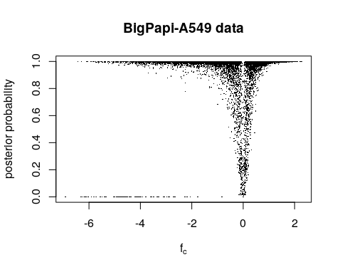
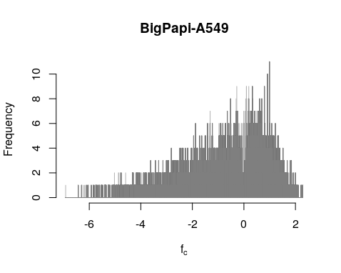
Using the first important function fit_ac_fc(), we establish the initial fc values (averaged over both replicates): fc = Cov(Xct)/Var(t). The posterior probability is the 1 minus q-value of t-test p-value of fc between pDNA and endpoint. We can see the valley of the posterior probability is not center at fc == 0. That is quite puzzling.
Part 2: modeling gene-gene interaction $\pi$
### Iterative Robust Least Squares Fitting ###
u1<-rep(0,nn)
names(u1)<-rownames(goodX)
u1[!allbad]<-1  #all other weights set to 1
fc0<-fc
fc_0<-matrix(0,nrow=nprobes,ncol=nprobes)
sdfc_0<-matrix(0,nrow=nprobes,ncol=nprobes)
w0_0<-matrix(0,nrow=nprobes,ncol=nprobes)
pp_0<-matrix(0,nrow=nprobes,ncol=nprobes)
rownames(fc_0)<-probes
colnames(fc_0)<-probes
rownames(sdfc_0)<-probes
colnames(sdfc_0)<-probes
rownames(w0_0)<-probes
colnames(w0_0)<-probes
rownames(pp_0)<-probes
colnames(pp_0)<-probes
for (i in 1:length(cpA)){
  construct<-paste(cpA[i], cpB[i], sep=";")
  w0_0[cpA[i],cpB[i]]<-u1[construct] #initial weights. non-existent pairs will have w0=0
  pp_0[cpA[i],cpB[i]]<-pp_fc[construct] #initial weights. non-existent pairs will have w0=0
  fc_0[cpA[i],cpB[i]]<-fc0[construct]
}

w0_0<-w0_0+t(w0_0) #make symmetric
fc_0<-fc_0+t(fc_0)
pp_0<-pp_0+t(pp_0)
Here we prepare all the matrix from the posterior obtained from fit_ac_fc(). In particular fc0_0, w0_0, sdfc_0 and pp_0 are probes vs probes pairwise matrices. w0_0 described whether the sgRNA-pair have passed the low-abundance threshold. pp_0 stored the posterior probability values and fc0_0 stored the estimated fitness fc. Now we are ready to model $\pi$ using the fc0 values.
irls<-function(fc,w0,probes,ag=2,tol=1e-3,maxiter=30) {
  # res2<-irls(fc_0,w0_0,probes,ag=2,tol=1e-3,maxit=50)
  # w0 is the physical goodness of constructs. It is not subject to change.
  # It is used to modify w, to silence bad constructs
  expressed_utri<-upper.tri(fc) & w0>0 ### at upper triangle in the matrix and passed low abundance threshold.
  n<-dim(fc)[1] ### no. of probes
  w<-matrix(1,nrow=n,ncol=n) #initial weights
  diag(w)<-0
  fij<-matrix(0,nrow=n,ncol=n) #initial weights
  eij<-matrix(0,nrow=n,ncol=n) #initial weights
  b<-rep(0,n) #rhs
  #iteration step 0
  w<-w*w0
  A<-w
  for (i in 1:n) {
    b[i]<-sum(fc[,i]*w[,i]) ### fc values (whole column) of a probe * low-abundance threshold column)
    A[i,i]<-sum(w[,i])+small ### diagonal cells, sgRNA1==sgRNA2
  }
  y<-solve(A,b) ### A = diagonal matrix, b fc values vector - solve for fc of a probe?
  names(y)<-probes
  for (i in 1:(n-1)) {
    for (j in (i+1):n) {
      fij[i,j]<-y[i]+y[j] ### addictive fc effects for 2 probes
    }
  }
  fij<-fij+t(fij)
  eij<-fc-fij #residuals ( in other words, errors)

  l<-1 #counter
  rel<-1
  while (rel > tol & l < maxiter) {#iterate until rel (relative errors) < tolerated value is reached or maxit
    s<-sd(eij[expressed_utri]) #calculate sd only from expressed constructs
    yold<-y
    w<-(1-eij^2/(ag*s)^2)^2 #something like Tukey's biweight
    w[abs(eij)>(ag*s)]<-0 # if error value too big, give 0 weight #
    diag(w)<-0

    w<-w*w0
    A<-w
    for (i in 1:n) {
      b[i]<-sum(fc[,i]*w[,i])
      A[i,i]<-sum(w[,i])+small ###add pseudo counts
    }
    y<-solve(A,b) ### A=matrix at LHS, b is result vector at RHS, solve the linear system which will return fc for each probe.
    names(y)<-probes
    fij<-matrix(0,nrow=n,ncol=n) #initial weights
    for (i in 1:(n-1)) {
      for (j in (i+1):n) {
        fij[i,j]<-y[i]+y[j]### addictive effect of 2 sgRNAs
      }
    }
    fij<-fij+t(fij)
    eij<-fc-fij #residuals: difference between fij (additive of solved fc (y)) compared to empirical fc data.

    rel<-sqrt(sum((y-yold)^2)/max(1,sum(yold^2))) #relative error
    cat(l,sqrtsum(yold),sqrtsum(y-yold),"\n")
    l<-l+1
  }
  vl<-list(y, fij, eij)
  return(vl)
}

#robust fitting
res2<-irls(fc_0,w0_0,probes,ag=2,tol=1e-3,maxit=50)
fp<-res2[[1]] ### == fij
mnull<-mean(fp[1:16]) ### fp of all sgRNA-pair containing at least 1 negative control
fp<-fp-mnull
fc<-fc-mnull*2
The function approximate y (predicted fc) through updating the w weight matrix with eij values in each iteration. Next we find the probes that give high fitness impact fc.
#find best probes
fp12<-data_frame(sgRNA=names(fp), fp=fp)
fp12$gene<-sapply(fp12$sgRNA, function(s) str_split(s, "_")[[1]][1])
fp12<-fp12 %>% group_by(gene) %>% mutate(rank_f=rank(-abs(fp))) #looking for the best (biggest abs value ==1)
rownames(fp12)<-fp12$sgRNA
rank_p<-fp12$rank_f
names(rank_p)<-probes

### wpi1 matrix return the rank sgRNA1 * rank sgRNA2
wpi1<-matrix(0,nrow=nprobes,ncol=nprobes)
rownames(wpi1)<-probes
colnames(wpi1)<-probes
for (i in 1:length(cpA)) {
    wpi1[cpA[i],cpB[i]]<-as.numeric(fp12[fp12$sgRNA==cpA[i], "rank_f"]*fp12[fp12$sgRNA==cpB[i], "rank_f"])
  }
Next fc of a gene is derived from the fc of sgRNAs * rank_f (not sure why high fc has less weight).
### find fitness for each gene
f<-rep(0,n)
names(f)<-genes
f<- fp12 %>% group_by(gene) %>% summarize(f=sum(rank_f*fp)/sum(rank_f)) %>% dplyr::select(f)
f<-unlist(f)
names(f)<-genes
fmean<-f ### mean gene fitness *weight
Now, we look at $\pi$ values between genes.
pi1<-res2[[3]] #raw pi-scores per construct
mean_pi1<-matrix(0,nrow=n,ncol=n)
rownames(mean_pi1)<-genes
colnames(mean_pi1)<-genes
goodX$cpA<-cpA
goodX$cpB<-cpB
for (i in genes){
  for (j in genes){
    probes_gene1<-probes[grepl(i, probes)]
    probes_gene2<-probes[grepl(j, probes)]
    expressed1<-c()
    local_w1<-c()
    local_pi1<-c()
  for (g in probes_gene1){
    for(h in probes_gene2){
      expressed1<-c(expressed1, w0_0[g,h]>0) ### check if low-abundance
      local_w1<-c(local_w1, wpi1[g, h]) ### look up sgRNA rank
      local_pi1<-c(local_pi1, pi1[g, h]) ### get pi score from each sgRNA from irls()
    }
      }
    local_w1<-local_w1/sum(local_w1[expressed1])*sum(expressed1)
    mean_pi1[i,j]<-sum((local_pi1*local_w1)[expressed1])/max(small,sum(local_w1[expressed1]))
  }
  }
Finally, we iterate the irls() function for n=iter times to get better estimate of $\pi$.
#### fit f for 5 iterations
###
##
#
uutri<-upper.tri(mean_pi1)
zi1<-mean_pi1[uutri]
zi<-zi1
npi<-length(zi1)
mmm<-length(fp)
niter=5
pi_iter<-matrix(0,nrow=npi,ncol=niter)
fp_iter<-matrix(0,nrow=mmm,ncol=niter)
f_iter<-matrix(0,nrow=n,ncol=niter)
rownames(f_iter)<-genes
utri<-upper.tri(fc_0)
ntri<-sum(utri)
ppi_iter<-matrix(0,nrow=ntri,ncol=niter)
for (iter in 1:niter) {
  cat("\n",iter,"\n")
  fc_1<-matrix(0,nrow=nprobes,ncol=nprobes)
  colnames(fc_1)<-probes
  rownames(fc_1)<-probes
  fc0<-fc_0[utri]+rnorm(ntri,sd=sdfc_0[utri]) ### update fc values with random variables ###
  pp0<-pp_0[utri]
  ### bootstraping data by randoming subseting some fc values
  draw<-ifelse(runif(ntri)<pp0,1,0)
  fc_1[utri]<-fc0*draw
  fc_1<-fc_1+t(fc_1)
  #robust fitting
  res2<-irls(fc_1,w0_0,probes,ag=2,tol=1e-3,maxit=50)
  fp0<-res2[[1]] #these are probe fitnesses fp
  mnull<-mean(fp0[1:16])
  fp0<-fp0-mnull

  for (i in genes) {
    w1<-(rank_p[grepl(i, names(rank_p))])^2 #ansatz for weights
    f_iter[i,iter]<-sum(w1*fp0[grepl(i, names(fp0))])/sum(w1) #weighted mean
  }
  pi1<-res2[[3]] #raw pi-scores per construct
  #rownames(pi1)<-probes
  #colnames(pil1)<-probes
  mean_pi1<-matrix(0,nrow=n,ncol=n)
  rownames(mean_pi1)<-genes
  colnames(mean_pi1)<-genes
  for (i in genes){
    for (j in genes){
      probes_gene1<-probes[grepl(i, probes)]
      probes_gene2<-probes[grepl(j, probes)]
      expressed1<-c()
      local_w1<-c()
      local_pi1<-c()
      for (g in probes_gene1){
        for(h in probes_gene2){
          expressed1<-c(expressed1, w0_0[g,h]>0)
          local_w1<-c(local_w1, wpi1[g, h])
          local_pi1<-c(local_pi1, pi1[g, h])
        }
      }
      local_w1<-local_w1/sum(local_w1[expressed1])*sum(expressed1)
      mean_pi1[i,j]<-sum((local_pi1*local_w1)[expressed1])/max(small,sum(local_w1[expressed1]))
    }
  }
  zi1<-mean_pi1[uutri]
  pi_iter[,iter]<-zi1
  fp_iter[,iter]<-fp0
}
Finally, we summarize all fc values across iterations and output result.
### summarize all iterations
f_mean<-apply(f_iter,1,mean)
f_sd<-apply(f_iter,1,sd)
fp_mean<-apply(fp_iter,1,mean)
fp_sd<-apply(fp_iter,1,sd)
pi_mean<-apply(pi_iter,1,mean)
pi_sd<-apply(pi_iter,1,sd)
pi_iter_null<-pi_iter-pi_mean
pi_null<-c(pi_iter_null,-pi_iter_null)
enull<-ecdf(pi_null)
emean<-ecdf(pi_mean)
### Histogram of Pi Scores
rge<-range(pi_mean[!is.na(pi_mean)])
h<-hist(pi_mean,breaks=seq(rge[1]-0.002,rge[2]+0.002,by=0.002),main="",xlab=expression(pi["gg'"]),col="grey80",border=FALSE,probability=TRUE)
d<-density(pi_null[!is.na(pi_null)],bw=0.002)
lines(d,col="black")
rug(pi_mean)
box()
### Pi Score File Output
z<-pi_mean/sd(pi_mean[!is.na(pi_mean)])
pi_iter_null<-pi_iter-pi_mean
abspi<-abs(pi_mean)
PP<-apply(abs(pi_iter_null)<abspi,1,mean)
oPP<-order(z)

#get names of these gene pairs
names_of_g1<-g1names[uutri]
fg1<-f[names_of_g1]
names_of_g2<-g2names[uutri]
fg2<-f[names_of_g2]
fg12<-fg1+fg2
names_of_gg<-ggnames[uutri]
fdr_left<-pmin(1,enull(pi_mean)/emean(pi_mean))
fdr_right<-pmin(1,(enull(-pi_mean))/(1-emean(pi_mean)))
plot(pi_mean,fdr_left,ylim=c(0,1),xlab=expression(pi["gg'"]),ylab="FDR, left") #left tail test
plot(pi_mean,fdr_right,ylim=c(0,1),xlab=expression(pi["gg'"]),ylab="FDR, right") #right tail test
res<-data.frame(names_of_gg,names_of_g1,fg1,names_of_g2,fg2,fg12,pi_mean,pi_sd,PP,abspi,fdr_left,fdr_right,z)
colnames(res)<-c("gene_gene","geneA","fA","geneB","fB","fA+fB","pi","sd","PP","abs_pi","FDR left","FDR right","z")
project=c("/path/to/dual_crispr_pipeline/bigpapi_A549")
write.table(res[oPP,],file=paste(project,"_pi.txt",sep=""),sep="\t",row.names=FALSE,quote=FALSE)
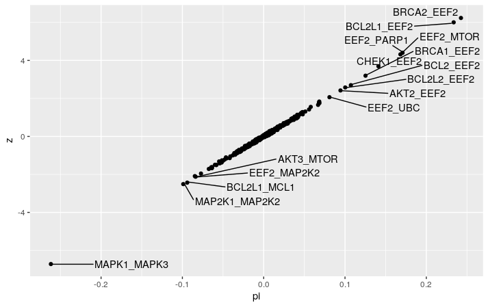
We can now plot the $\pi$ values, and see that the MAPK1-MAPK3 pair stands out as expected to be the strongest interacting gene pair. We also observed the BCL2L1-MCL1 pair mentioned in the Gemini paper. Interestingly, we have EEF2 interacting with all sort of genes, mainly positively. This is not mentioned in the Gemini paper at all.
GEMINI
GEMINI takes a different approach, focusing on the LFC that the observed LFC of a sgRNA pair gi and hj: Dgi,hj is derived from 3 latent factors: x-technical noise where it is named as sample-independent errors, y-individual gene KO effect, and s-combined effect of double KO.
Normal priors are set up for x($\mu$=1, $\sigma$=1), y($\mu$=0, $\sigma$=10) and s($\mu$=0, $\sigma$=10); individual and combined gene KO effects are expected to be 0 with a small portion of genes giving huge impact (thus $\sigma$=10). In addition, a parameter $\tau$ is used for fitting the LFC for each guide pair.
GEMINI use coordinate ascent variational inference (CAVI) to estimate all parameters x, y, s, and $\tau$. From the gemini_inference() function, it looks like that x is updated first, followed by y, s, and $\tau$ at last.
Finally, a GEMINI score for each gene pair is calculated. It is a relative score of the additional combine effect of double KO compared to the highest effect of the individual gene.
| sgene1,gene2 | - max( | Ygene1 | , | Ygene2 | ) |
The commands of GEMINI are very simple.
library("gemini")
data("counts", "guide.annotation", "sample.replicate.annotation", package = "gemini")
Input <- gemini_create_input(counts.matrix = counts,
                             sample.replicate.annotation = sample.replicate.annotation,
                             guide.annotation = guide.annotation,
                             ETP.column = 'pDNA',
                             gene.column.names = c("U6.gene", "H1.gene"),
                             sample.column.name = "samplename",
                             verbose = TRUE)
Input %<>% gemini_calculate_lfc(normalize = TRUE,
                                CONSTANT = 32)
### normalise with median LFC value ###
Model <- gemini_initialize(Input = Input,
                           nc_gene = "CD81",
                           pattern_join = ';',
                           pattern_split = ';',
                           cores = 1,
                           verbose = TRUE)
Model %<>% gemini_inference(cores = 1,
                            verbose = FALSE)

gemini_plot_mae(Model)
nc_pairs <- grep("6T|HPRT", rownames(Model$s), value = TRUE)
Score <- gemini_score(Model = Model,
             pc_gene = "EEF2",
             nc_pairs = nc_pairs)
The modeling is done through gemini_initialize() and gemini_inference(). Looking into the Model object, there are lists for variable x (172 row = 172 individual probes), xx (array of 7128 sgRNA pairs), lists for y (28 row = 28 genes), and lists of s (378 rows = 378 gene pairs). $/tau$ is stored as two tables: alpha and beta.
It is quite interesting to dig through the raw codes in the GIMINI github. I could see that the influence is done through updating x first, then y, s and $/tau$ consecutively. The code is very clean and easy to read. It is very helpful for me to learn about writing Bayesian functions!
The final results are generated in the gemini_score(). Of note, the positive gene (pc_gene) used here is EEF2. That validated our previously dual_cripr_pipeline results.
In the Score object, gene-gene interaction score seems to be stored in the $strong table – a combined result from table sensitive_lethality and sensitive_recovery.
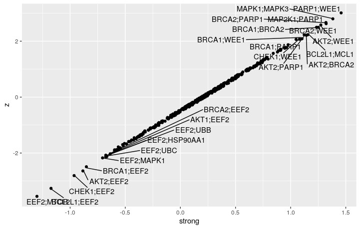
We can see that GEMINI discovered a lot more interacting gene pairs compared to the dual_crispr_pipline. I wonder is that because more replicates in different cell line are used. And the gemini score and $/pi$ are of opposite signs. Indeed, if I only use pDNA and A549 counts for GEMINI, the model did not converge unless I have raise the convergence threshold to 0.01.
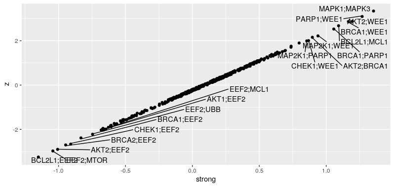
Still, most of the strong interacting gene pairs are preserved while only using the A549 samples.
Conclusion
Both dual_crispr_pipline and GEMINI both have show consistent results. Although GEMINI is easier to use, the dual_crispr_pipline allow us to analyse time-series count data. In that sense, I think we shall use both pipeline and compare results to get more confident on the gene-gene interaction hits. Finally, it is so very cool that both pipeline publish their codes and have organised that in a clearly written and easy-to-adopt manner. I have learnt some new ways to do modeling in R for linear systems and updating models.