New way to find DEGs in scRNA-seq

Single-cell studies is shifting focus. Instead of grouping cells into neat cluster, theres are more about the transcriptomes and dynamics in the data that portrait the cell state in a more truthful way. This is what SingleCellHaystack(Vandenbon A, Diez D (2020) aims at, to find defining DEGs without the underlying cluster assumptions.

Transition from clusterings

Defining groups of cells to infer cell type identity is an indispensable step in single-cell sequencing analysis. The workflow usually consists of a cell x gene matrices consists of the informative genes (highly variable genes) decompose via PCA and present in 2D via t-SNE or UMAP. From there, k-means clustering is performed to identify groups of cell subtypes. Then the ingroup against all other cells would be tested (i.e. FindAllMarkes function in Seurat) to assign gene markers for each group.

Here, SingleCellHaystack adopt a different approach to identify important DEGs. After obtaining the 2D or multi-dimension decomposition of the gene matrix of single cells, it look into where cells (all express a gene/ do not express that gene) are in the multi-dimensional space.

In brief, in a dimension from (i.e. PCA), 100 grid points are assigned to cover the distribution of all the cells. For a grid point i, the euclidean distance of cells from i are measured. The full distance distribution of all genes (Q) is compared to the distribution of cells that have a particular gene (G) expressed or not (P(G=T) and P(G=F)). The Kullback–Leibler Divergence between the null model Q and the distribution of cells (G=T)/(G=F) is computed. The higher the KD divergence indicates the higher importance of the gene G contributing to the spatial patterns of the cells in the PCs.

Implementation of SingleCellHaystack

The documentation of SingleCellHaystack is quite detailed and easily followed. I am using the multi-dimension application for this post. SingleCellHaystack requires two input: the dimension reduction embeddings of cells, and a matrix indicating whether gene expression is detected or not ((G=T) and (G=F)) in each cell.

Here, I used the PBMC dataset provided by Seurat tutorial as our test data.

I ran Seurat and SingleCellHaystack in parallel and compared the final results.

library(dplyr)
library(Seurat)
library(patchwork)
pbmc.data <- Read10X(data.dir = "/media/achu/新增磁碟區/book notes/2020-09-11-haystack/filtered_gene_bc_matrices/hg19")
pbmc <- CreateSeuratObject(counts = pbmc.data, project = "pbmc3k", min.cells = 3, min.features = 200)
pbmc <- NormalizeData(pbmc, normalization.method = "LogNormalize", scale.factor = 10000)
pbmc <- FindVariableFeatures(pbmc, selection.method = "vst", nfeatures = 2000)
pbmc <- ScaleData(pbmc)
pbmc <- RunPCA(pbmc, features = VariableFeatures(object = pbmc), npcs=50)
pbmc <- RunUMAP(pbmc, dims = 1:50)
pbmc.markers <- FindAllMarkers(pbmc, only.pos = TRUE, min.pct = 0.25, logfc.threshold = 0.25)

From Seurat, I obtained the 1) normalised expression matrix, 2) a list of highly variable genes, 3) PCA analysis results of 50 PCs, and 4) Umap analysis results. I use the normalised expression matrix of the highly variable genes and the PCA results for SingleCellHaystack.

library(ggplot2)
library(singleCellHaystack)
median.per.gene <- apply(as.matrix(pbmc@assays$RNA@data)[pbmc@assays$RNA@var.features, ],1,median) 
pbmc.detection <- as.matrix(pbmc@assays$RNA@data)[pbmc@assays$RNA@var.features, ]> median.per.gene 
###2000 genes x 2700 cells ###

### try to run haystack with Hd ###
pbmc.pc50 <- haystack(x = pbmc@reductions$pca@cell.embeddings[,1:50], detection = pbmc.detection, method = "highD")
show_result_haystack(res.haystack = pbmc.pc50, n = 10)
#D_KL log.p.vals log.p.adj T.counts
#FCGR3A 0.001751152  -57.76185 -54.46082      497
#LGALS2 0.001500851  -55.92850 -52.62747      573
#CST7   0.001427542  -54.19082 -50.88979      535
#IFI30  0.001818254  -53.60855 -50.30752      441
#SPI1   0.001362165  -53.34830 -50.04727      571
#CFD    0.001442612  -52.90949 -49.60846      616
#GZMA   0.001346472  -52.79575 -49.49472      541
#CD79A  0.001864891  -52.66374 -49.36271      426
#CCNB2  5.277959312  -52.54073 -49.23970        4
#LY6G6F 2.552268293  -51.59671 -48.29568        8
res.top <- show_result_haystack(res.haystack = pbmc.pc50, n = 1000)
res.top$rank<-rank(res.top$log.p.adj)
g<-left_join(pbmc.markers,
          res.top %>% mutate(gene=rownames(res.top)), by="gene")

Here, SingleCellHaystack has returned a list of the top 1000 DEGs. The table indicates the significances of the KL divergence of a gene compared to the null model and the number of cells (T.count) with that gene expressed.

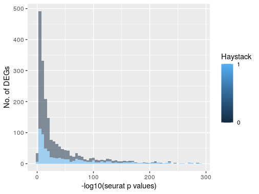
When I compared the results of SingleCellHaystack 1000 DEGs to Seurat gene markers (2024 genes detected) from FindAllMarkers(), the top 14 genes with the lowest p values in Seurat is also within the 1000 DEGs from SingleCellHaystack (ranking from 2 to 200). In Seurat results, 88 gene markers are ribosomal genes, most are markers belonging to cluster 0. These ribosomal genes are not supposed to be DEGs, and SingleCellHaystack successful filter out all but 3 of them. This indicates that SingleCellHaystack may be more sensitive then Seurat.

Furthermore, among the top 1000 DEGs from SingleCellHaystacks (blue in figure, Haystack=1), most shared a significant p values (<0.01) in Seurat. In that light, SingleCellHaystacks appears to be a reliable tool to detect DEGs.

Furthermore, these DEGs are allow to distribute across clusters which show a more complex but non-static picture of the SingleCell data. It shows that SingleCellHaystack will give us a higher resolution in transcriptomic dynamics among cells compared to the widely-adopted rigid clustering methods.

Therefore, it will be useful to run SingleCellHaystack on top of others packages to refine the DEG list.