Using MAUDE.

Pooled CRISPR library screens have become a very popular tool for forward genetic screens that study transcriptional regulation, enhancer elements and pathway components, etc. Although, CRISPR-i is ways more effective than sgRNA inhibition, CRISPR efficiency is highly dependent on the sgRNA, both on its activity and specificity. Therefore, it is important to benchmark how effective a sgRNA is in delivering it desired phenotype. Previously, ScreenProcessing scripts (developed based on the concept of Kampmann et al (2013)) has been used for quantification of sgRNA effect on pooled library that were keep at exponential growth phrase. ScreenProcessing aimed at determining the difference between the growth rate of a particular CRISPR knockdown compared to the WT. The net growth rate of the CRISPR mutant is referred as the phenotypic effect ($\gamma). Negative $\gamma indicates growth inhibition; positive $\gamma shows growth promoting effects and $\gamma equals to 0 means an absence of effect (same as WT (untreated control)). ScreenProcessing usually process pooled CRISPR deep sequencing data that the abundance of a sgRNA are proximate to the read count in the population at several time points over the course of exponential growth(t₀, t₁, t₂…).

ScreenProcessing are useful for sgRNA targeting genes that produce phenotypes (changes in growth rate), but may not be useful if the sgRNA target do not alter growth but rather change a reporter expression such as fluorescence in a GFP-disruption assay. That’s where the new package MAUDE comes in handy.

MUADE: Mean Alterations Using Discrete Expression

In brief, MAUDE spcialises on CRISPR screens that result in a reporter readout that reflective to the sgRNA effect. The reporter expression (i.e. fluorescence) are then used for generating FACS data that have subpopulations of cells sorted into different bins based on the reporter expression. Based on the deep sequencing data of the unsorted and sorted bins and their population compositions, MAUDE assign the sgRNA effect by comparing the read count enrichment to those of the non-targeting sgRNAs. Using the non-targeting sgRNAs to establish a baseline effect distribution, MAUDE then report a Z-score for individual sgRNA effect.

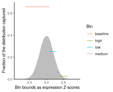
Here, we try out the MAUDE tutorial on the CD69 CRISPR-a experiment (Simeonov et al (2017)). The author engineer CRISPR-a throughout a 135 kb region upstream of CD69, sorted transduced cells based on their CD69 expression level and measured the distribution of gRNAs in the sorted populations. In the experiment, we have baseline, low, medium and high bins with the background unsorted population, in total 5 set of deep sequencing data.

library(openxlsx)
library(reshape)
library(ggplot2)
library(MAUDE)
library(GenomicRanges)
library(ggbio)
library(Homo.sapiens)

CD69Data = read.xlsx('https://www.ncbi.nlm.nih.gov/pmc/articles/PMC5675716/bin/NIHMS913084-supplement-supplementary_table_1.xlsx')

#identify non-targeting guides
CD69Data$isNontargeting = grepl("negative_control", CD69Data$gRNA_systematic_name)

CD69Data = unique(CD69Data) # for some reason there were duplicated rows in this table - remove duplicates
CD69Data = unique(CD69Data) # for some reason there were duplicated rows in this table - remove duplicates

#reshape the count data so we can label the experimental replicates and bins, and remove all the non-count data
cd69CountData = melt(CD69Data, id.vars = c("PAM_3primeEnd_coord","isNontargeting","gRNA_systematic_name"))
cd69CountData = cd69CountData[grepl(".count$",cd69CountData$variable),] # keep only read count columns
cd69CountData$Bin = gsub("CD69(.*)([12]).count","\\1",cd69CountData$variable)
cd69CountData$expt = gsub("CD69(.*)([12]).count","\\2",cd69CountData$variable)
cd69CountData$reads= as.numeric(cd69CountData$value); cd69CountData$value=NULL;
cd69CountData$Bin = gsub("_","",cd69CountData$Bin) # remove extra underscores

There were two biological replicates in the data. After all the re-organisation of the dataframe, we have the final key columns specifying sgRNA details, replicate number, bin, and read count.

#reshape into a matrix
binReadMat = data.frame(cast(cd69CountData[!is.na(cd69CountData$PAM_3primeEnd_coord) | cd69CountData$isNontargeting,], 
                             PAM_3primeEnd_coord+gRNA_systematic_name+isNontargeting+expt ~ Bin, value="reads"))
dhsPeakBED = read.table(system.file("extdata", "Encode_Jurkat_DHS_both.merged.bed", package = "MAUDE", mustWork = TRUE), 
                        stringsAsFactors=FALSE, row.names=NULL, sep="\t", header=FALSE)
names(dhsPeakBED) = c("chrom","start","end");
#add a column to include peak names
dhsPeakBED$name = paste(dhsPeakBED$chrom, paste(dhsPeakBED$start, dhsPeakBED$end, sep="-"), sep=":")dhsPeakBED = read.table(system.file("extdata", "Encode_Jurkat_DHS_both.merged.bed", package = "MAUDE", mustWork = TRUE),       stringsAsFactors=FALSE, row.names=NULL, sep="\t", header=FALSE)
names(dhsPeakBED) = c("chrom","start","end");
#add a column to include peak names
dhsPeakBED$name = paste(dhsPeakBED$chrom, paste(dhsPeakBED$start, dhsPeakBED$end, sep="-"), sep=":")

#read in the bin fractions derived from Simeonov et al Extended Data Fig 1a and the "digitize" R package
#Ideally, you derive this from the FACS sort data. 
binStats = read.table(system.file("extdata", "CD69_bin_percentiles.txt", package = "MAUDE", mustWork = TRUE), 
                      stringsAsFactors=FALSE, row.names=NULL, sep="\t", header=TRUE)
binStats$fraction = binStats$binEndQ - binStats$binStartQ; #the fraction of cells captured is the difference in bin start and end percentiles

Then you also have the location of the sgRNA targets in the BED file dhsPeakBED and the bin fractions details from the FACS @ binStats$fraction.

#convert bin fractions to Z scores
binStats$binStartZ = qnorm(binStats$binStartQ)
binStats$binEndZ = qnorm(binStats$binEndQ)

ggplot(binStats, aes(colour=Bin))  + 
  geom_density(data=data.frame(x=rnorm(100000)), aes(x=x), fill="gray", colour=NA)+ 
  ggplot2::geom_segment(aes(x=binStartZ, xend=binEndZ, y=fraction, yend=fraction)) + 
  xlab("Bin bounds as expression Z-scores") + 
  ylab("Fraction of the distribution captured") +theme_classic()+scale_y_continuous(expand=c(0,0))+
  coord_cartesian(ylim=c(0,0.7))

binStats = rbind(binStats, binStats) #duplicate data
binStats$expt = c(rep("1",4),rep("2",4)); #name the first duplicate expt "1" and the next expt "2";

guideLevelStats = findGuideHitsAllScreens(experiments = unique(binReadMat["expt"]), 
                                          countDataFrame = binReadMat, binStats = binStats, 
                                          sortBins = c("baseline","high","low","medium"), 
                                          unsortedBin = "back", negativeControl = "isNontargeting")

findGuideHitsAllScreens function of MAUDE runs MAUDE and return all the sgRNA effects in a corrected Z-score. The results showed the sgRNA effect (mean column) and the centered sgRNA effect (Z column).

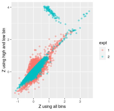
By testing the results of gRNA effect using only the high and the low bins compared to using all four bins for the learning, we can see that Z scores learnt from only using the low and high bins are in general over-estimated; and inaccuracy are exacerbated when Z score get larger than 3.

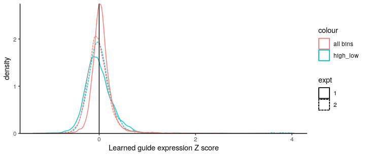
Interestingly, Z score cannot be centered if using only two bins of the data (even with 4478 non-targeting control sgRNA). It may be due to the fact that the fractions of the two bins (low=25%, high=2.8%) are not big enough for accurate normalisation.

Still, it will be good to see that there will be a further development that enable us to have better inferences with fewer bins, as most labs typically can afford to sequence the unsorted background vs the selected bin of highest reporter expression.