Why and how to merge single-cell experiments?

There is a trend of increasing re-sequencing projects as well as comparative genomics projects in the single-cell field. With the pressing demands to bridge the past studies to the newly sequenced data for scientific discovery, a few leading labs are rolling out benchmarking guidelines and new packages to integrate single-cell experiments from numerous technologies and multiple experimental conditions.

I am looking into several batch-correction/integration methods in this post, in the hope to understand more of the mathematical concepts behinds and have a educated guess on which of these methods may be best for my data.

My urge to think more deeply about integration stemmed from my colleague pointing out to me that 10x data is generally overwhelmed with mitochondria and ribosomal transcripts. It did not matter much for highly differential populations as the marker genes driving the clustering are highly expressed and differ greatly between cell types. However, transcriptome profiles do not differ that drastically in my personal project; the dominating cluster markers are mitochondria and ribosomal genes. Removing them from the analysis will give me even more ambiguous results and I start questioning whether what I see is a technical artifacts from 10x or these genes are truly differentially expressed in the experimental condition I am studying. More importantly, do these so-called “markers” behave similarly if different sequencing technologies will be implemented? I have to kind of come up with a proposal of what is the sensible next step as my collaborators are reluctant to spend money on bulk-RNAseq to validate these “markers genes” I found in the 10x data.

So I decided to look into what people have done so far about comparing results from different technologies, especially about integration. Here, I have tried out Seurat, Combat, scran fastMNN, limma removebatcheffect(), liger and BEER, to see how they perform on integrating the benchmarking SCRNA-seq data of the pancreas generated from CelSeq, CelSeq2 and SMART-Seq2 (from Seurat tutorial). I aimed to find out 1: what integration has achieved from these methods? 2: how the integrated data is used in the downstream analysis.

Seurat integration pipeline (v3)

Of course, starting with the easiest, we first look into the Seurat integration pipeline. In summary, Seurat use the hvg found in multiple experiments, identify the “anchors” (‘two cells (with one cell from each dataset), that we predict to originate from a common biological state.’), find the genes with shared CCA loadings using the “anchors” and then put the KNN-neighbors between anchors together during the dimension reduction steps. In the paper, it stresses that the step of anchors identification is key to successful integration and lets see what Seurat returns from the dataset.

library(Seurat)
library(ggplot2, dplyr)
options(future.globals.maxSize = 4000 * 1024^2)
pancreas.data <- readRDS(file = "/home/a/Documents/trails_errors_bioinformatics/Batch_effects_correactions/pancreas_v3_files/pancreas_expression_matrix.rds")
metadata <- readRDS(file = "/home/a/Documents/trails_errors_bioinformatics/Batch_effects_correactions/pancreas_v3_files/pancreas_metadata.rds")
pancreas <- CreateSeuratObject(pancreas.data, meta.data = metadata)
pancreas.list <- SplitObject(pancreas, split.by = "tech")

### now there are 4 dataset ###
### SCTransform : retrurn vst corrected counts, data=log1p(corrected counts), scaled.data:pearson residuals### 
for (i in 1:length(pancreas.list)) {
  pancreas.list[[i]] <- SCTransform(pancreas.list[[i]], verbose = FALSE)
}

pancreas.features <- SelectIntegrationFeatures(object.list = pancreas.list, nfeatures = 500)
### cannot run the following as there are not enough space ###


pancreas.list <- PrepSCTIntegration(object.list = pancreas.list, anchor.features = pancreas.features, 
                                    verbose = FALSE)
pancreas.anchors <- FindIntegrationAnchors(object.list = pancreas.list, normalization.method = "SCT", 
                                           anchor.features = pancreas.features, verbose = FALSE)
pancreas.integrated <- IntegrateData(anchorset = pancreas.anchors, normalization.method = "SCT", 
                                     verbose = FALSE)

pancreas.integrated <- RunPCA(pancreas.integrated, verbose = FALSE)
pancreas.integrated <- RunUMAP(pancreas.integrated, dims = 1:30)
plots <- DimPlot(pancreas.integrated, group.by = c("tech", "celltype"), combine = FALSE)
plots <- lapply(X = plots, FUN = function(x) x + theme(legend.position = "top") + guides(color = guide_legend(nrow = 3,  byrow = TRUE, override.aes = list(size = 3))))
CombinePlots(plots)
rm(pancreas.data, pancreas.integrated, pancreas.list)

Seurat UMAP from anchoring 500 hvg genes

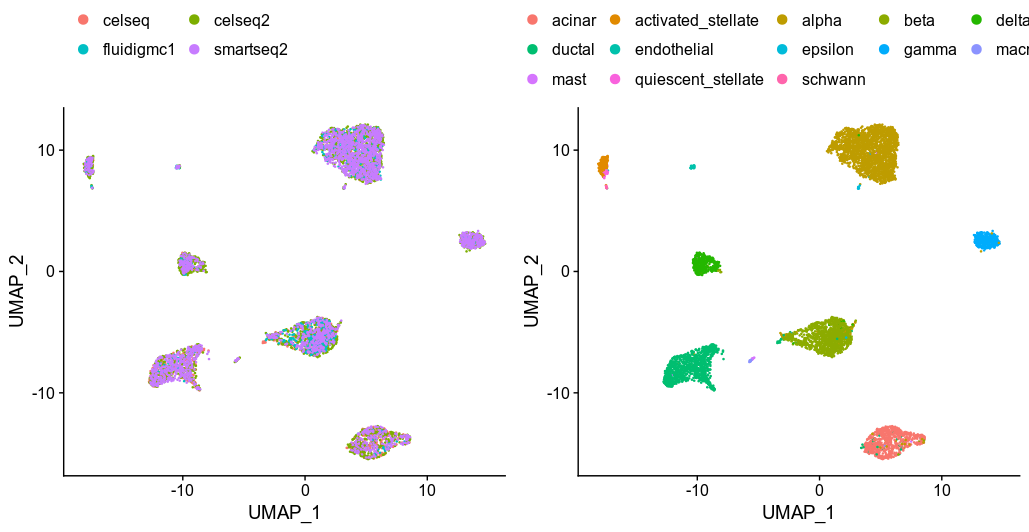
Seurat returns the corrected expression values of these 500 selected hvg genes, generated the UMAP from the PCA results of the corrected expression matrix and perfectly merge the data. Seurat argued that the CCA methods is more robust compare the fastMNN as it can handle different cell-type compositions among dataset. So the next thing to test is scran/batchelor fastMNN.

fastMNN

### set up dataset ###
library(scater)
library(scran)
library(batchelor)

names<-dimnames(pancreas.data)
celseq<-SingleCellExperiment(assays=list(counts=pancreas.list$celseq@assays$RNA@counts))
celseq2<-SingleCellExperiment(assays=list(counts=pancreas.list$celseq2@assays$RNA@counts))
smartseq2<-SingleCellExperiment(assays=list(counts=pancreas.list$smartseq2@assays$RNA@counts))
rm(pancreas.list, pancreas)
### use the pancreas.features identified by seurat ###
###  try scran fastMNN ###
### assume that two batches contain at least one common cell type, and that the batch effect is orthogonal to the biological differences in each batch
normalised_combined<-batchelor::multiBatchNorm(celseq, celseq2, smartseq2, assay.type="counts", min.mean = 1)
in.all <- Reduce(intersect, list(rownames(celseq), 
                                 rownames(celseq2), rownames(smartseq2)))

logcounts(celseq)<-normalised_combined[[1]]@assays$data[["logcounts"]]
logcounts(smartseq2)<-normalised_combined[[3]]@assays$data[["logcounts"]]
logcounts(celseq2)<-normalised_combined[[2]]@assays$data[["logcounts"]]
combined<-scran::fastMNN(celseq, celseq2, smartseq2, k=20, approximate=TRUE, subset.row=in.all)
library(Rtsne)
combined_tSNE<-Rtsne(combined$corrected, pca=F)
plot(combined_tSNE$Y, col=c(rep(1, 1004), rep(2, 2285), rep(3, 2394)), main="scran-fastMNN")
legend("topleft", legend=c("celseq", "celseq2", "smartseq2"),
       col=c(1, 2, 3), horiz=TRUE, cex=0.8, pch=1, box.lwd=0.5, bg=NULL)
exp_tab<-data.frame(combined_tSNE$Y)
colnames(exp_tab)<-c("x", "y")
rownames(exp_tab)<-c(rownames(colData(celseq)), rownames(colData(celseq2)), rownames(colData(smartseq2)))
exp_tab<-cbind(exp_tab, metadata[rownames(exp_tab), ])

library(cowplot)
p1<-exp_tab %>% ggplot((aes(x=x, y=y, colour=tech)))+ geom_point()+theme(legend.position = "top")+guides(fill=guide_legend(ncol=1))
p2<-exp_tab %>% ggplot((aes(x=x, y=y, colour=celltype)))+ geom_point()+theme(legend.position = "top")
plot_grid(p1, p2 )

fastMNN tSNE from the 50 PCs derived from fastMNN

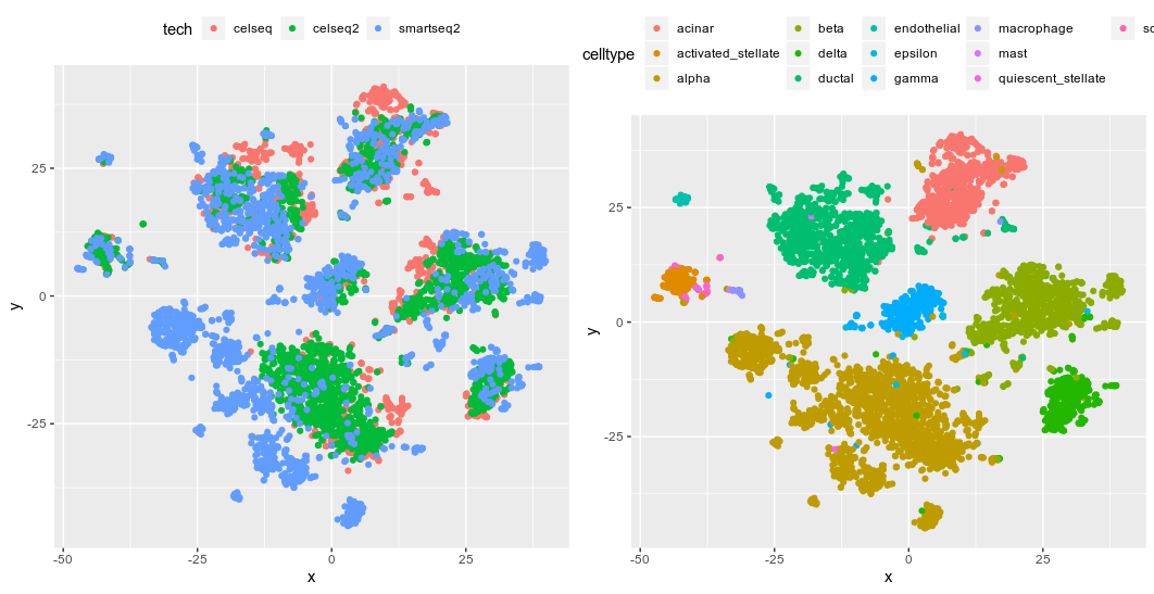
I have to say that I have a lot of issues with the updating to the latest version of bioconductor, scran and scater; there were a few missing commands until I have every version of software correct. The good thing about fastMNN is that it returns the corrected expression values for every gene (via multiplying the gene-loading matrix to the cell-loading matrix). So I can have a look at how other gene expression had changed due to the correction, which is not available in other methods. The clustering is decent except for the alpha cells, which is the biggest group of cells in the dataset. Maybe it is also the noisiest (more cells, more diversity?) subpopulation that compromised the fastMNN. Well, some cells end up having negative expression values; probably because they had low RNA counts to begin with. The author says that it is okay as the expression values shall not be interpreted as logcounts, and I guess we can still calculate DE via these corrected expression values?

Combat and limma

Next we turn to the other two popular correction methods, ComBat() from the SVA package and removeBatchEffect() from limma. Limma is just a correction of each gene per batch using a linear model with a design matrix. ComBat removes the batch effects by modelling and removing the effect of the latent factor. Both limma and ComBat required log and normalised data from input. In ComBat, genes needed to be further filtered with expression variance bigger than 0.

### SVA Combat
library(sva)
library(scater)
library(limma)
### setup data ###
### Combat crash before for prarmetric estimation, but took too long for non-prarmetric ones ###
keep_genes<-apply(pancreas.data, 1, var)!=0
keep_cells<-rownames(metadata[metadata$tech %in% c("celseq", "celseq2", "smartseq2"), ])
pancrease_sce<-SingleCellExperiment(assay=list(counts=pancreas.data[keep_genes, keep_cells]),
                                    colData=metadata[keep_cells, ])
library(scRNAseq)
pancrease_sce<-computeSumFactors(pancrease_sce)
pancrease_sce<-scater::logNormCounts(pancrease_sce)
pancrease_norm<-as.matrix(logcounts(pancrease_sce))
pancrease_norm<-pancrease_norm[rowSums(pancrease_norm)>1, ]
### lowered to 24074 genes ###

### try to use Combat on log2 data ###
###  Users are returned an expression matrix that has been corrected for batch effects. The input data are assumed to be cleaned and normalized before batch effect removal. 
### try to see removing genes has variance of 0 can evade the error
pancrease_combat<-ComBat(pancrease_norm, batch=colData(pancrease_sce)$tech, prior.plots=T, mod=NULL)
combats_results<-colSums(pancrease_combat)
### Error in while (change > conv) { : missing value where TRUE/FALSE needed
### remove features with low variances, have NA exp or too many 0?? ###
pos_cells<-names(combats_results[combats_results>=10])
### normalised combat results return all positives exp values ###
pancrease_sce<-SingleCellExperiment(assay=list(logcounts=pancrease_combat[, pos_cells]), colData=metadata[pos_cells, ])
pancrease_sce<-scater::calculatePCA(pancrease_sce, ncomponents = 50,
                                    ntop = 2000)
library(Rtsne)
pancrease_tSNE<-Rtsne(pancrease_sce, pca=F)
combat_tsne<-pancrease_tSNE$Y
rownames(combat_tsne)<-pos_cells
colnames(combat_tsne)<-c("x", "y")
combat_tsne<-cbind(combat_tsne, metadata[pos_cells, ])
library(cowplot)
library(ggplot2)
library(dplyr)
p1<-combat_tsne %>% ggplot((aes(x=x, y=y, colour=tech)))+ geom_point()+theme(legend.position = "top")+guides(fill=guide_legend(ncol=1))
p2<-combat_tsne%>% ggplot((aes(x=x, y=y, colour=celltype)))+ geom_point()+theme(legend.position = "top")
plot_grid(p1, p2 )
### limma ###
### again input log2 size-normalised gene exp matrix ###
### no design matrix, given as there were no treatment conditions differed except the batch effects ###
pancreas_limma<-removeBatchEffect(pancrease_norm, batch = metadata[pos_cells, "tech"])
### return A numeric matrix of log-expression values with batch and covariate effects removed ###
### again use the corrected matrix for sce clustering ###
pancrease_sce<-SingleCellExperiment(assay=list(logcounts=pancreas_limma[, pos_cells]), colData=metadata[pos_cells, ])
pancrease_sce<-scater::calculatePCA(pancrease_sce, ncomponents = 50,
                                    ntop = 500)
pancrease_tSNE<-Rtsne(pancrease_sce, pca=F)
limma_tsne<-pancrease_tSNE$Y
rownames(limma_tsne)<-pos_cells
colnames(limma_tsne)<-c("x", "y")
limma_tsne<-cbind(limma_tsne, metadata[pos_cells, ])
p1<-limma_tsne %>% ggplot((aes(x=x, y=y, colour=tech)))+ geom_point()+theme(legend.position = "top")+guides(fill=guide_legend(ncol=1))
p2<-limma_tsne%>% ggplot((aes(x=x, y=y, colour=celltype)))+ geom_point()+theme(legend.position = "top")
plot_grid(p1, p2 )

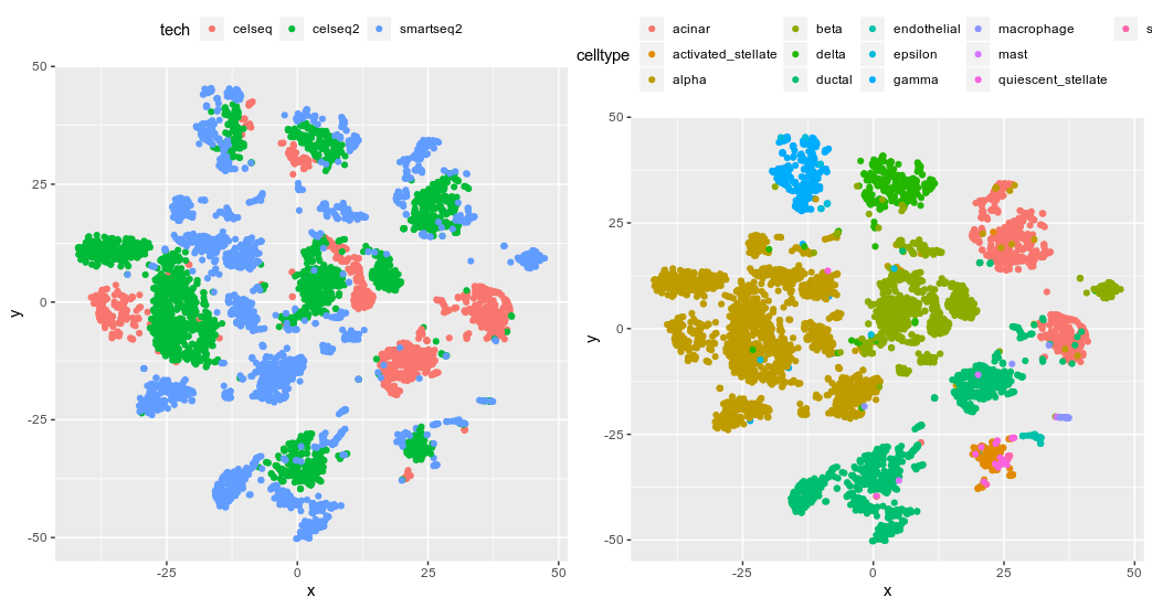
ComBat tSNE from the 50 PCs build from 2000 top hvg

limma tSNE from the 500 top hvg

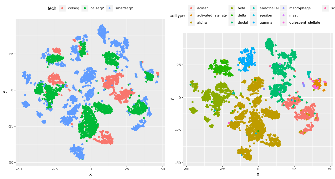
We can clearly see that both methods did a poor job in integrating the data across all cell types. That is kinda surprising considering how popular they are.

factorization with liger

liger uses NNMF to identify shared metagenes across dataset. Then the integration was done by putting cells with similar loadings to the metagenes into the same cluster (pretty much?).

library(liger)
celseq_cells<-rownames(metadata[metadata$tech=="celseq", ])
celseq2_cells<-rownames(metadata[metadata$tech=="celseq2", ])
smartseq2_cells<-rownames(metadata[metadata$tech=="smartseq2", ])  

ligerex <- createLiger(list(celseq = pancreas.data[, celseq_cells] , celseq2 = pancreas.data[, celseq2_cells], smartseq2=pancreas.data[, smartseq2_cells])) #Can also pass in more than 2 datasets
ligerex <- normalize(ligerex)
ligerex <-selectGenes(ligerex)
### found 16977 var genes ###
ligerex <- scaleNotCenter(ligerex)
### estimate no. of factors useful for aligning the datasets
k.suggest <- suggestK(ligerex, k.test = seq(5, 50, 10), num.cores = 1, gen.new = T, return.data = T, plot.log2 = T,
                      nrep = 5)
### integrate datasets via the quantile alignment step ###
### identifies similarly loading cells across datasets by building a similarity graph based on shared factor neighborhoods
### Using Louvain community detection, we then identify clusters shared across datasets, and align quantiles within each cluster and factor

### optimizeALS is the factorization step that return the H W V matrix for each dataset ###
ligerex <- optimizeALS(ligerex, k=25, thresh = 5e-5, nrep = 3)
### 15 cell types, but look like the KL divergence slows down at k=25 ###
ligerex <- quantileAlignSNF(ligerex, resolution = 0.4, small.clust.thresh = 50)
### forgo small cluster, aim to align the big ones ###
ligerex <- runTSNE(ligerex)
liger_tsne<-ligerex@tsne.coords
colnames(liger_tsne)<-c("x", "y")
liger_tsne<-cbind(liger_tsne, metadata[rownames(liger_tsne), ])
# Modify plot output slightly
library(ggplot2)
library(dplyr)
p1<-liger_tsne %>% ggplot((aes(x=x, y=y, colour=tech)))+ geom_point()+theme(legend.position = "top")+guides(fill=guide_legend(ncol=1))
p2<-liger_tsne%>% ggplot((aes(x=x, y=y, colour=celltype)))+ geom_point()+theme(legend.position = "top")
plot_grid(p1, p2 )

liger tSNE from the 25 metagenes

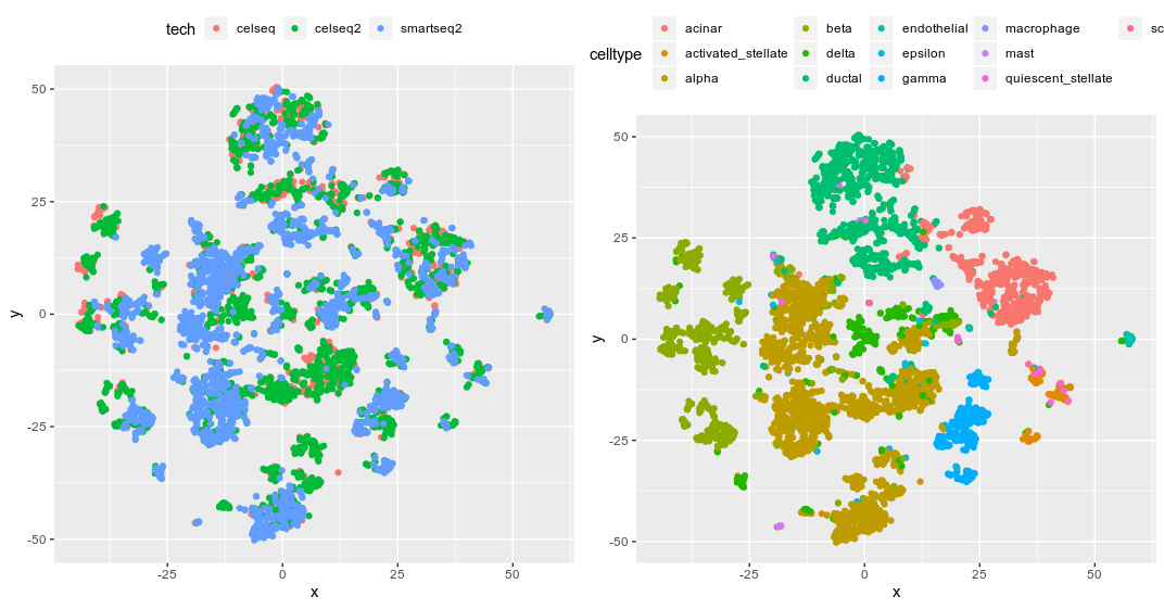
I have to say the liger performance is the worst; some cell types got mixed up and the clusterings of the beta cells scatter across the plot. There might be room for improvements if I try different k (metagenes) to model.

BEER

Finally, I tried this newly published method BEER. The idea behind it is neat, it looked for highly correlated PCs across dataset, and only use those PCs for clustering. It even has the potential to combine differently type of experiment such as acATAC-seq and scRNA-seq.

library(Seurat)
### guess feed the scaled data from Seurat to BEER? ###
### II. Combine Multiple Batches ###
pancreas_beer<-BEER(pancreas.data[, c(celseq_cells, celseq2_cells, smartseq2_cells)], metadata[c(celseq_cells, celseq2_cells, smartseq2_cells), ]$tech, GNUM=30, PCNUM=50, ROUND=1, GN=2000, SEED=1, COMBAT=TRUE)

# Check selected PCs #
PCUSE=pancreas_beer$select
COL=rep('black',length(pancreas_beer$cor))
COL[PCUSE]='red'
plot(pancreas_beer$cor,pancreas_beer$lcor,pch=16,col=COL,
     xlab='Rank Correlation',ylab='Linear Correlation',xlim=c(0,1),ylim=c(0,1),
     main="BEER highly correlated PCs")
### 44 highly correlated PCs ###
pancreas_beer_seurat<-pancreas_beer$seurat
pancreas_beer_seurat@meta.data$cell_type<-metadata[rownames(pancreas_beer_seurat@meta.data), ]$celltype
pancreas_beer_seurat<- RunUMAP(pancreas_beer_seurat, dims = 1:30)
plots <- DimPlot(pancreas_beer_seurat, group.by = c("batch", "cell_type"), combine = FALSE)
plots <- lapply(X = plots, FUN = function(x) x + theme(legend.position = "top") + 
                  guides(color = guide_legend(nrow = 3, byrow = TRUE, override.aes = list(size = 3))))
CombinePlots(plots)

BEER UMAP from 44 correlated PCs

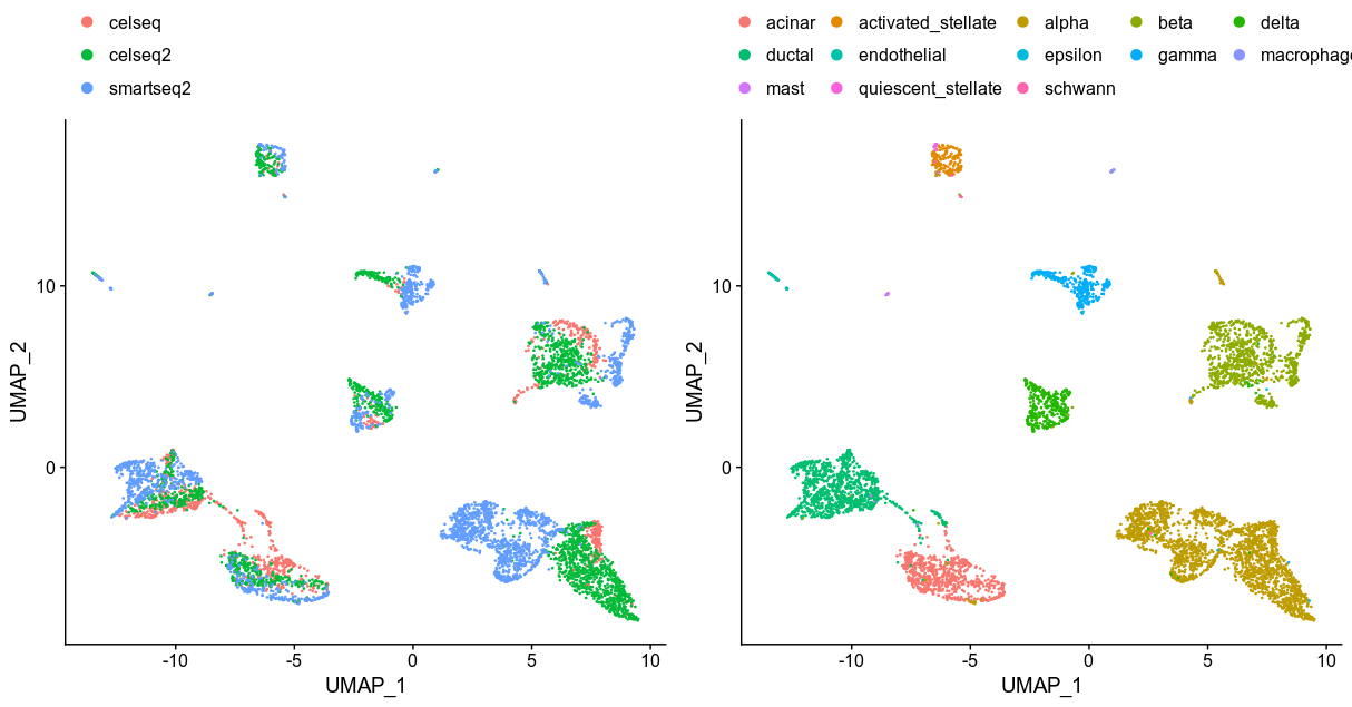
BEER found 44 highly correlated PCs and used them for integration. It returned the corrected expression and final integrated PCA in a Seurat object. I just needed to directly run UMAP and I have to say the clustering is comparable to Seurat; still the alpha cells are not clustered well. It seems like a persisting challenge for all the packages tested so far. ### Conclusion We examined a few integration methods and so far Seurat integration pipeline did best. fastMNN and BEER performed well and provide the full corrected expression matrix, which may be useful for other downstream analyses. The main limitation for all of these methods is that they expect certain overlaps of cell types among data. This goes against some of the experimental designs that cells were FACS sorted to different batches and sequenced separately. Hopefully, the samples could be pooled for sequencing in future experiments using the new antibodies-tagging procedures such as ECCITE-seq to circumvent the problem. Data integration would definitely become the essential step in future single-cell studies as more data will be jointly analysed. However, so far with the available technology, integration methods was still focusing on accurate clustering. Once the cell is successfully labeled, the dataset has to be split again for DE analyses among clusters. This works well so far for cells with clear differentiation profiles, but not so much for cells that share signatures with more than one cell-types (i.e. in transition states), which is quite common in development process. The common practice so far is to sequence at a temporal manner and stitches the data together in pseudo-time. But maybe data integration will provide a new approach to understand cellular development if we could truly merge the data together and interrogate cells that fall between well-defined clusters.