Pooling small-effect genes together to find signals

I have been reading NMF tutorials for a long time but didn’t quite understand it, since there were not a lot of examples that is biology related. Therefore, I am delighted to finally learn about it through its application on single-cell data.

The first paper that introduce the application of NMF on biological data that I read is by Gaujoux and Seoighe 2010 and Brunet et al 2004. And I going through the example in the paper (ALL vs AML data) using the NMF package in R was extremely helpful for figuring out how and why NMF is useful for charactering gene networks in expression datasets.

So basically, NMF models the number of factors (metagenes) for a group of cells. A cell’s expression profile is defined by a small number of metagenes, which made up of a group of genes with correlated expression pattern. The contribution of a gene to a metagenes is listed in the W matrix (gene x metagene matrix) and the contribution of each metagene to a cell expression profile is shown in the H matrix (factor x cell matrix). NMF returns a basis component (showing each gene contribution to a metagene) and a coefficient matrix (showing the loadings of each metagene in a cell). In some simple cases, the number of metagene reflects the number of clusters one expected in a population that cells within a cluster all share the same dominant metagene.

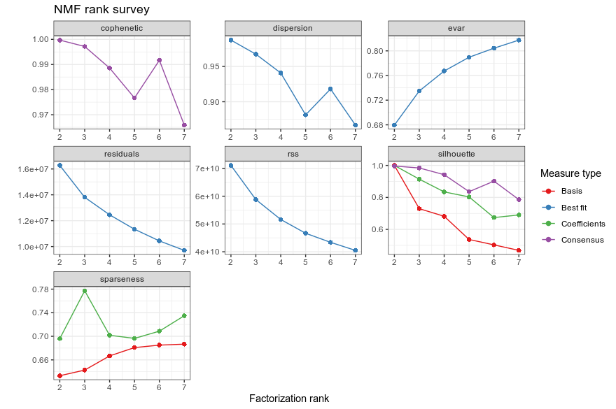
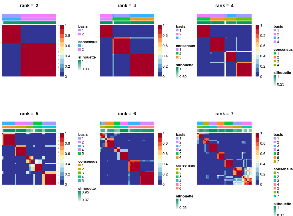
The ALL and AML data is an excellent example for NMF tutorial. NMF with two metagenes perfectly split the ALL from the AML patients. Increasing to three metagenes showed that ALL patients could be further split into two subtypes, fully consistent with the pathology. i also learnt a new term “cophenetic coefficient” (okay it shall not come as a stranger cause it is used in phylogenetics). It is a measure to test if the dendrogram (clustering splitting map) agrees with the cell-cell distance matrix. Base on the cophenetic coeff., sparseness and shihouette plot, using up to 4 metagene could lead to the best clustering (up to 4 clusters).

NMF of ALL vs AML patients

NMF consensus matrix of ALL vs AML patients

Further readings suggested that metagenes from NMF can be additive, so one can mix and match metagene loadings to reflect different cell stages/types. This concept is particularly attractive because cells can simultaneously undergo different programmes (differtiations and starving, for instance) and NMF potentially could separate the two programmes from the cells rather than defining these cells to be a new cell type.

Single-cell RNA-seq NMF

cNMF and scNBMF are both published this year (Sun et. al. 2019 and Kotliar et. al. 2019). Both methods explored different aspects of single-cell datausing NMF. scNBMF imputed gene expressions with a negative binomial distribution before factorization and it add an (LASSO) penalty component to the W matrix for repressed gene of a cell falsely possessed a read count. The package aims at increasing clustering accuracy (by finding metagenes that give the highest sparseness between clusters) and computing efficiency. cNMF, in contrast, aims to identifying Gene Expression programs (GEP) from complex expression profiles. The different compositions of the underlying metagenes explained the observed variations (aka clusterings) of cells. The impressive point of cNMF is that the output metagenes constitute of correlated genes (so likely to be co-expressed), and metagenes are as distant as possible from each other.

I used the brain data (GEO: GSE67835) consists of 466 brain cells and apply both methods on it for performance testing. I used scNBMF first because it was used by the original scNBMF paper and see if I could reconstruct the figure 2h in the paper.

### preprocessing the data ###
### put individual csv together to make a expression matrix ###
setwd("/path/to/folder/E-GEOD-67835.processed.1")
all_csv<-list.files(pattern="*.csv")
brain_data<-read.csv(all_csv[1], header = F, stringsAsFactors = T, row.names = 1, sep = "\t")
cell_name<-strsplit(all_csv[1], "\\.")[[1]][2]
colnames(brain_data)<-cell_name
for (i in 2:length(all_csv)){
  exp_per_cell<-read.csv(all_csv[i], header = F, stringsAsFactors = T, row.names = 1, sep = "\t")
  cell_name<-strsplit(all_csv[i], "\\.")[[1]][2]
  colnames(exp_per_cell)<-cell_name
  brain_data<-cbind(brain_data, exp_per_cell)
}
write.csv(brain_data,file="GSE67835-GPL15520_processed_mtx.csv", row.names = T, quote = F)
scNBMF("/GSE67835-GPL15520_processed_mtx.csv")

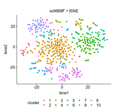
The script did not run till the end because I did not have the cell-type labels for the dataset; nonetheless it has generated the H_results.csv, which is the loading matrix of the cells. According to the paper, using the first 10 components was enough to produce a high resolution T-SNE; that’s not quite true. Finally, I used all 20 components for K-means clustering (k=10 as provided by the ground truth) and tSNE. The clustering still looks poor (no boundaries between clusters) but the clustering returns somewhat correct numbers for each group. But still I cannot reconstruct the tSNE of figure 2h.

scNBMF results

clusters 1 2 3 4 5 6 7 8 9 10

No. of cells 20 152 20 79 36 26 22 41 57 13

scNBMF metagenes=20 tSNE

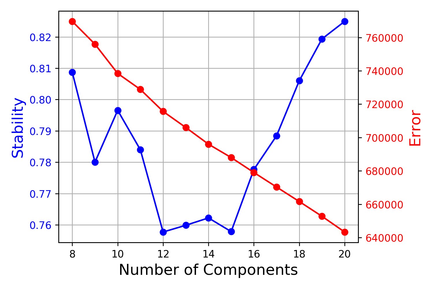
Next I run cNMF in conda env with the same data. I set -k from 8 to 20 to see what is the best k.

python ./cnmf.py prepare --output-dir /home/a/Documents/trails_errors_bioinformatics/2019_10_30_NMF_scRNA-seq/cNMF \
--name brain_data_normalised -c /home/a/Documents/trails_errors_bioinformatics/2019_10_30_NMF_scRNA-seq/E-GEOD-67835.processed.1/GSE67835-GPL15520_filtered_mtx.csv -k {8..20} --n-iter 100 --total-workers 1 --seed 14 --numgenes 2000

#Step 2 run NMF
python ./cnmf.py factorize --output-dir /home/a/Documents/trails_errors_bioinformatics/2019_10_30_NMF_scRNA-seq/cNMF \
 --name brain_data_normalised --worker-index 0 \
 --show-clustering -k {8..20} \
 --genes-file /home/a/Documents/trails_errors_bioinformatics/2019_10_30_NMF_scRNA-seq/cNMF/brain_data_normalised/brain_data_normalised.overdispersed_genes.txt

### Combine ###
python ./cnmf.py combine --output-dir /home/a/Documents/trails_errors_bioinformatics/2019_10_30_NMF_scRNA-seq/cNMF \
--name brain_data_normalised \
-k {8..20}

rm /home/a/Documents/trails_errors_bioinformatics/2019_10_30_NMF_scRNA-seq/cNMF/brain_data_normalised/cnmf_tmp/*spectra*iter*npz

python ./cnmf.py k_selection_plot \
--output-dir /home/a/Documents/trails_errors_bioinformatics/2019_10_30_NMF_scRNA-seq/cNMF \
--name brain_data_normalised

### cluster ###
python ./cnmf.py consensus --output-dir /home/a/Documents/trails_errors_bioinformatics/2019_10_30_NMF_scRNA-seq/cNMF \
--name brain_data_normalised \
--components (10/20) --local-density-threshold (0.01/0.1/2) --show-clustering

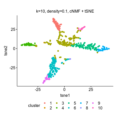
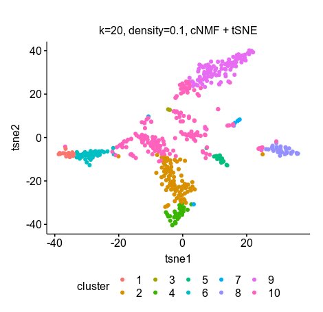
cNMF showed that using k=20 has the highest stability and lowest errors, but the consensus plots looks very strange that there are groups of cells sharing certain components (GEP). Finally, I picked k=20, density threshold=0.1 and K=10, density threshold=0.1 for the final results, as it has retained the highest information content.

scNBMF metagenes=20 tSNE

Then I input the usage.consensus.txt (the H matrix) in R for tSNE and k-means clustering (k=10). The clustering was closer to ground truth using 10 GEP for clustering compared to 20, and the tSNE showed better separations compared toe scNBMF.

cNMF results

k=10, density=0.1

clusters 1 2 3 4 5 6 7 8 9 10

No. of cells 46 1 134 32 82 102 30 2 22 15

k=20, density=0.1

clusters 1 2 3 4 5 6 7 8 9 10

No. of cells 6 32 27 164 90 80 4 14 34 15

scNMF GEP=10 density-threshold=0.1 tSNE

scNMF GEP=20 density-threshold=0.1 tSNE

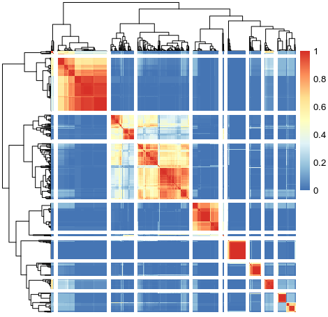
SC3 clustering kinda showed that clustering is difficult among two groups of brain cells that they shared fail amount of between-cluster similarity but enough differences to maintain as two clusters. This suggested that there are common underlying GEP shared between two different cell types.

SC3 consensus matrix k=10

The good thing about cNMF is that it also output the gene_spectra matrix for looking into the gene rank (importance) in each GEP for further analysis such as GO enrichment. It is more comprehensive if one is interest in finding regulatory circuits governing the cell phenotype or dealing with more complex data. The cNMF github page also provide very good documentation of all the analysis done in the paper and two tutorials for further downstream analyses, it is definitely worth digging further for investigating GEPs and how they interact and contribute to a cell’s expression profile.